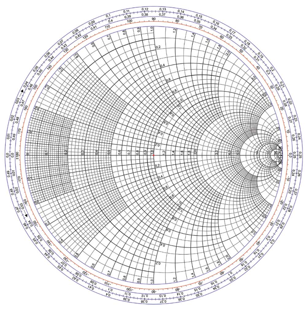
his is the first of the three articles devoted to the Smith Chart and the calculations of the input impedance to a lossless transmission line. This article begins with the load reflection coefficient and shows the details of the calculations leading to the resistance and reactance circles that are the basis of the Smith Chart. A sample Smith Chart is shown in Figure 1, [1].
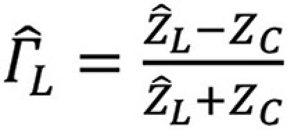
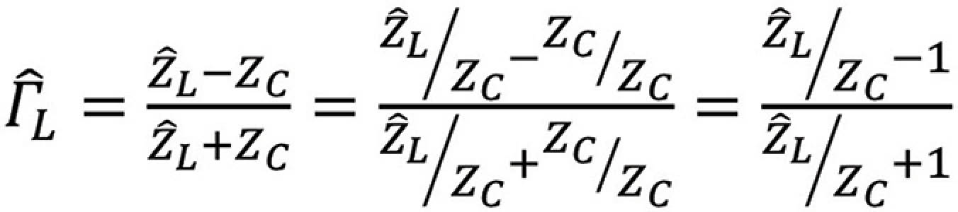
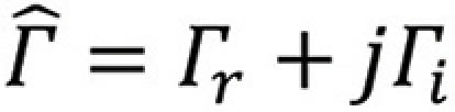
The load reflection coefficient, in either model, can be obtained directly from the knowledge of the load and the characteristic impedance of the line as
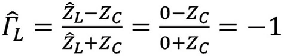
There are three special cases of the load reflection coefficient
 L = 0
L = 0
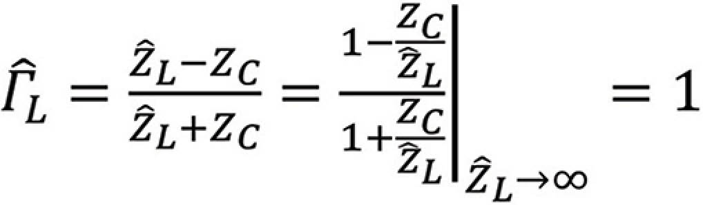
Open-Circuited Line, L = ∞
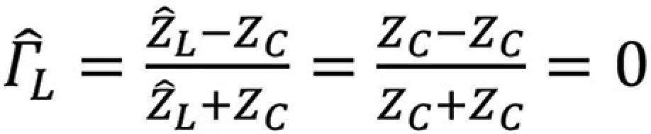
Matched Line, L = ZC
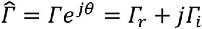
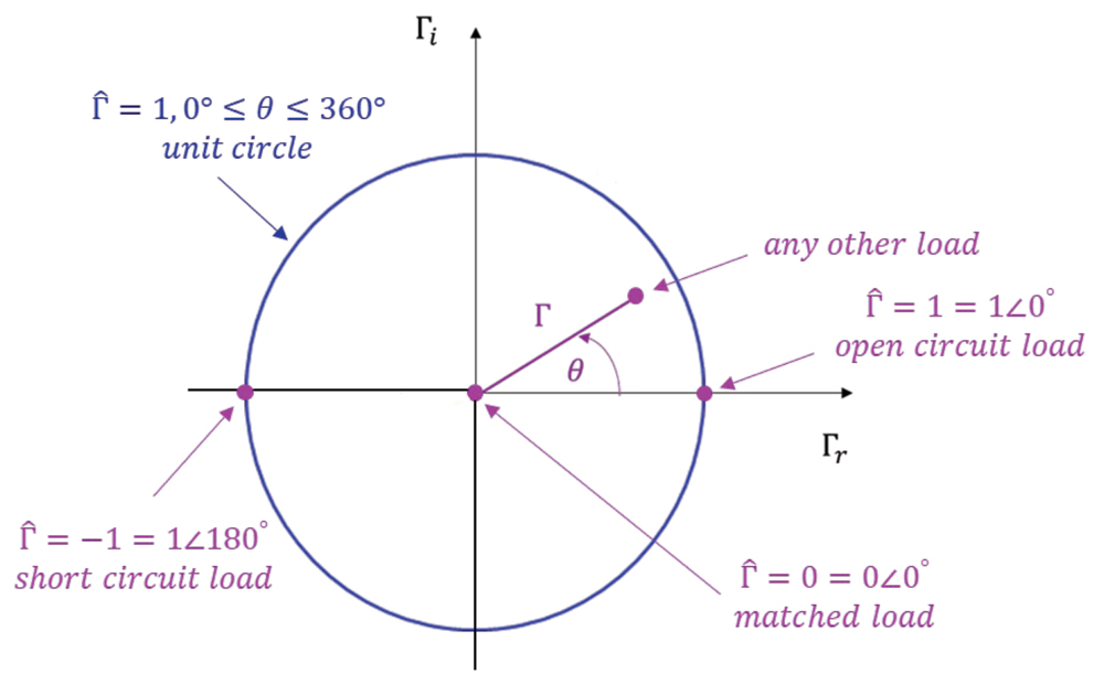
For passive loads, the magnitude of the load reflection coefficient is always
The magnitude of 0 (center of the complex plane) corresponds to a matched load, the magnitude of 1 with the angle of 0º represents an open circuit, while the magnitude of 1 with the angle of 180º represents a short circuit. Shown in Figure 4 is also a unit circle, which sets the boundary for all the points representing a passive load reflection coefficient.
or
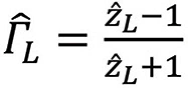
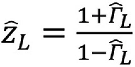
where the small letter  L denotes the normalized load impedance, i.e., L = L /ZC. Smith Chart is based on the plot of the load reflection coefficient utilizing this normalized load impedance, as explained next.
Multiplying both sides by the denominator of the right-hand side, we obtain
or
and thus
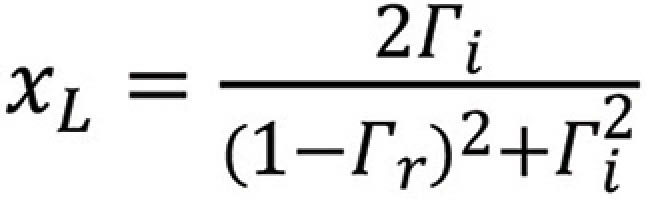
and finally,
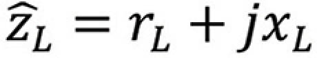
where rL is the normalized load resistance and xL is the normalized load reactance.
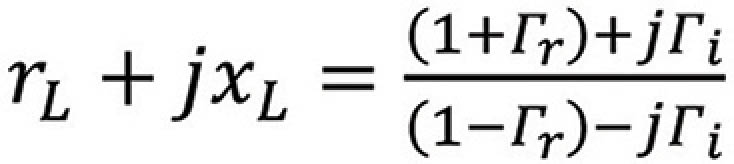

Multiplying out the terms in the numerator and grouping the real and imaginary part gives
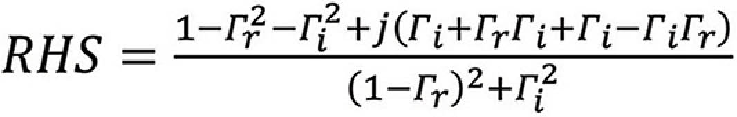
or
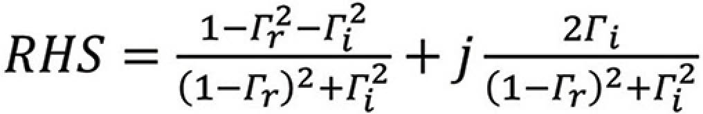
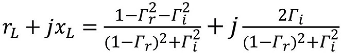
Equating the real and imaginary parts we get
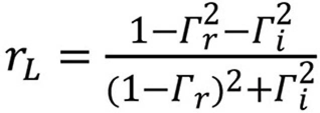

or

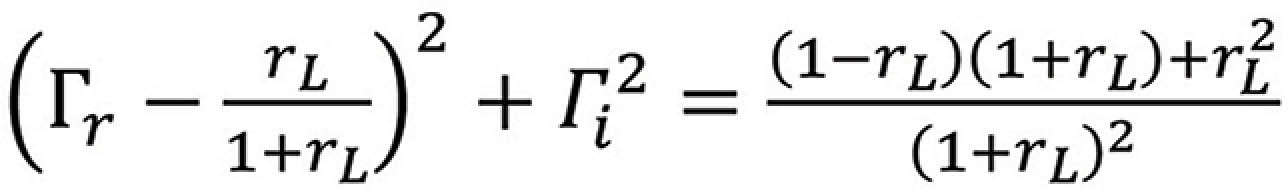
Multiplying out and rearranging we get

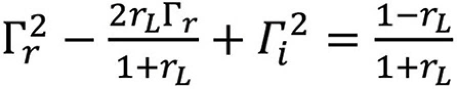
or

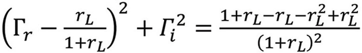
Dividing both sides by (1 + rL) we have
 to both sides results in
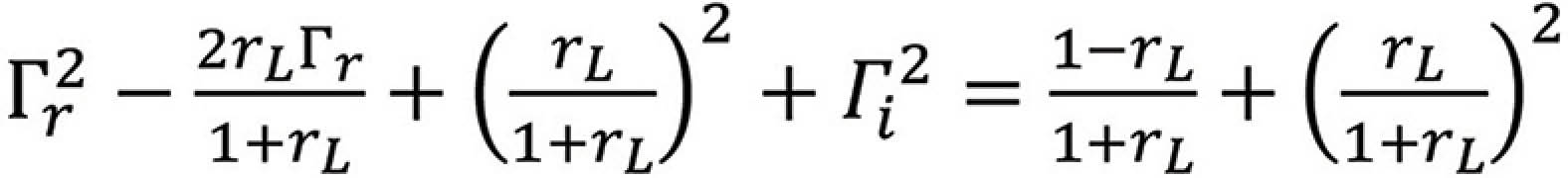
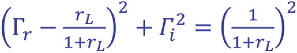
leading to
or
and finally,
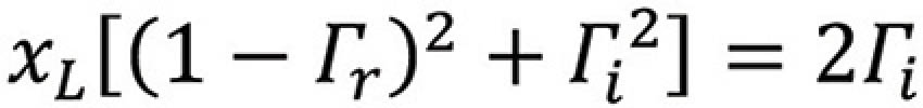
or
Multiplying out and rearranging we get

Dividing both sides by xL we have
leading to
Equations (3.23) and (3.29) have the form of
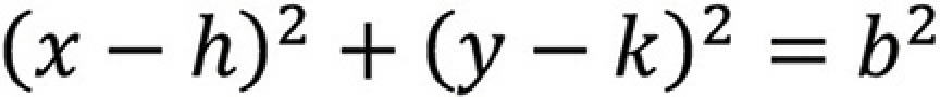
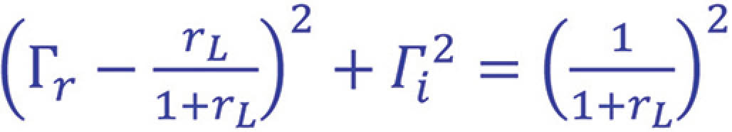
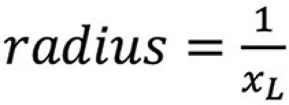
describes a circle in the ΓrΓi plane. This circle has a radius
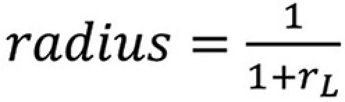
and is centered at
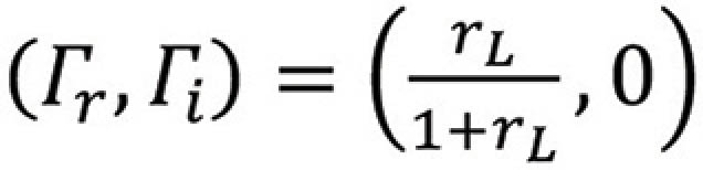
We refer to this circle as the resistance circle.
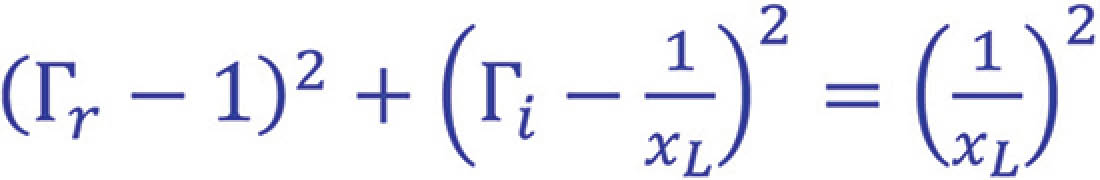
describes a circle of
centered at
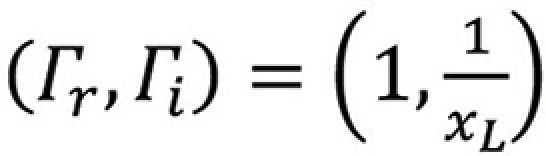
We refer to this circle as the reactance circle.
References
- https://upload.wikimedia.org/wikipedia/commons/7/7a/Smith_chart_gen.svg
- Adamczyk, B., “Sinusoidal Steady State Analysis of Transmission Lines – Part II: Voltage, Current, and Input Impedance Calculations – Circuit Model 1,” In Compliance Magazine, February 2023.
- Adamczyk, B., “Sinusoidal Steady State Analysis of Transmission Lines – Part III: Voltage, Current, and Input Impedance Calculations – Circuit Model 2,” In Compliance Magazine, March 2023.
- Adamczyk, B., “Sinusoidal Steady State Analysis of Transmission Lines – Part I: Transmission Line Model, Equations and Their Solutions, and the Concept of the Input Impedance to the Line,” In Compliance Magazine, January 2023.
