Sinusoidal Steady State Analysis of Transmission Lines
his is the second of the three tutorial articles devoted to the frequency-domain analysis of a lossless transmission line. In the previous article, [1], the general solution for the voltage and current in sinusoidal steady state was derived and the concept of the input impedance to the line was presented. This article shows numerous methods of calculating the voltage, current, and input impedance at various locations on the transmission line, using the Circuit Model 1, [1], described next.
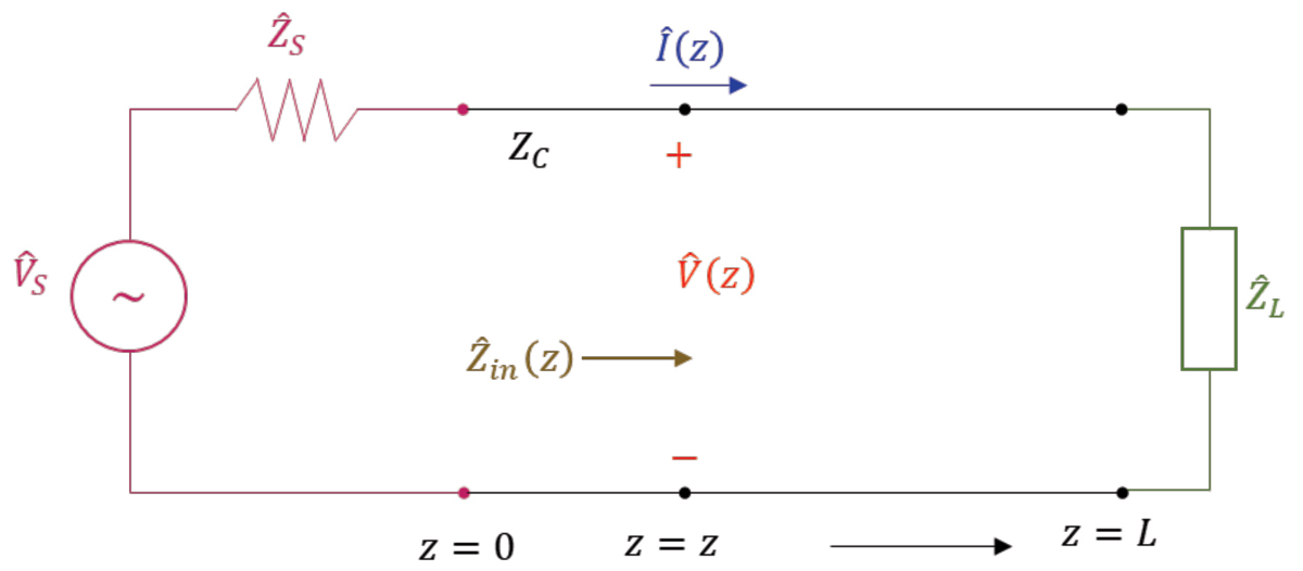
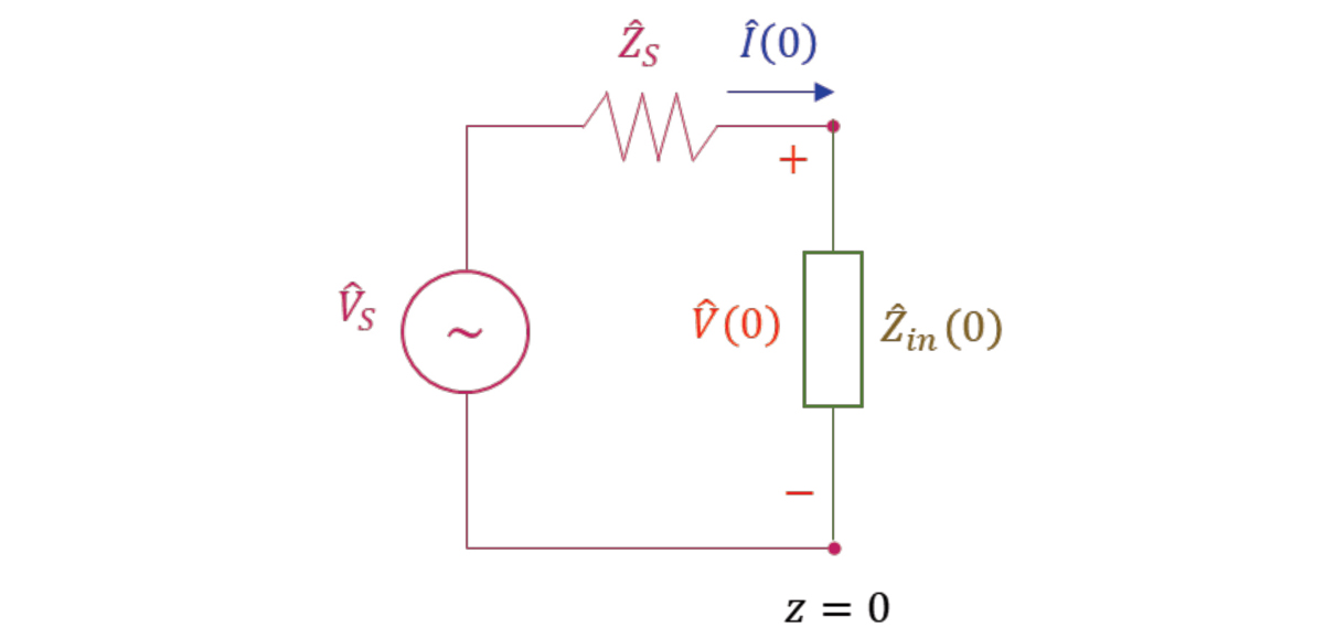
Consider a lossless transmission line with the characteristic impedance Zc, driven by the source located at z = 0 and terminated by the load located at z = L, as shown in Figure 1. (This circuit was referred to as Circuit Model 1, in [1]).
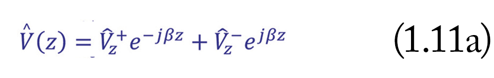
The voltage and current at any location z away from the source were derived in [1] as
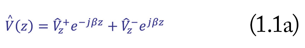
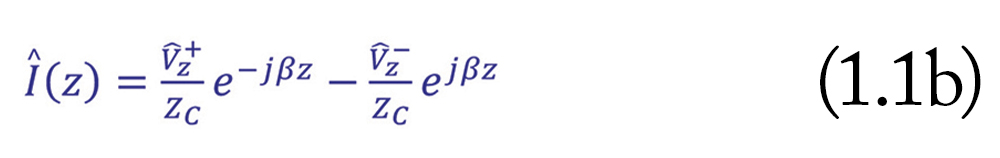
where β is the phase constant of the sinusoidal voltage source and the Vz+ and Vz– are yet to be determined constants.
Note: In [1] these constants were denoted as V+ and V-. Here, we use a different notation to distinguish between the constants for two different circuit models. Using Model 1, shown in Figure 1, we move from the source at z = 0 to the load at z = L, and use constants Vz+ and Vz–. In Model 2, discussed in the next article, we move from the load at d = 0 to the source at d = L, and use constants Vd+ and Vz–. These two sets of constants are different.
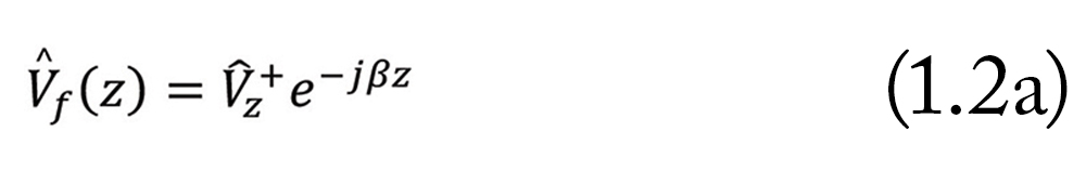
The solutions in Eqns. (1.1) consist of the forward- and backward-traveling waves. The forward-traveling voltage wave is described by
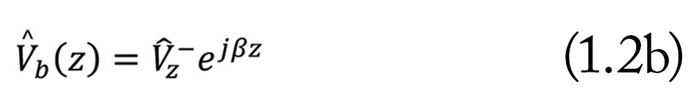
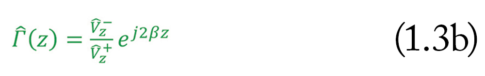
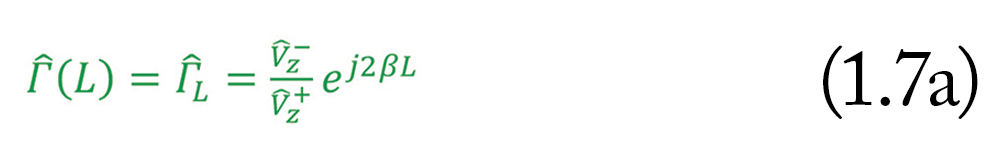
Using these two waves, we define the voltage reflection coefficient at any location z, as the ratio of the backward-propagating wave to the forward-propagating wave
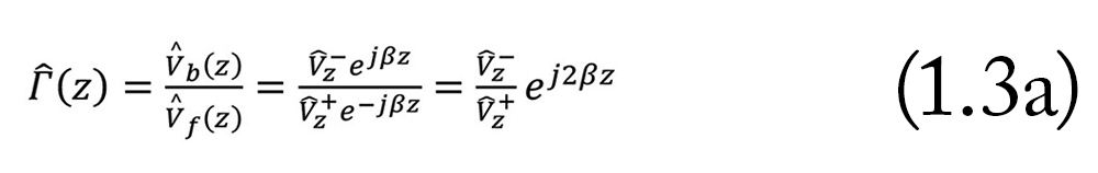
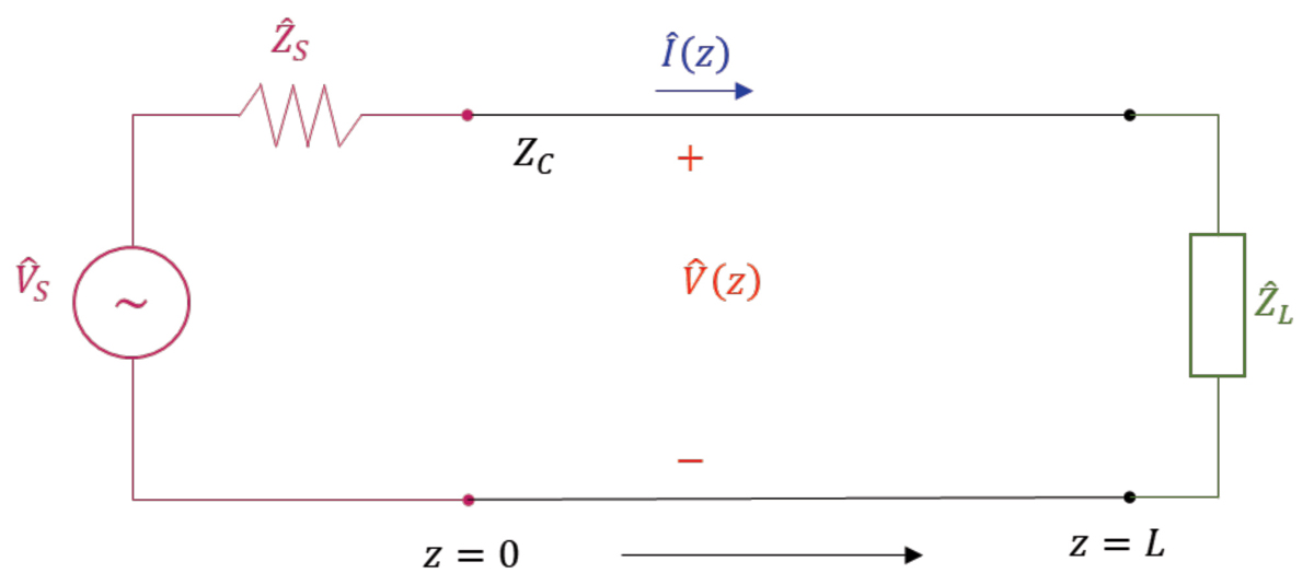
Figure 1: Transmission line circuit with the source located at z = 0 and the load at z = L
Thus,
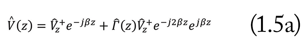
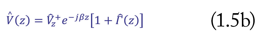
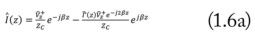
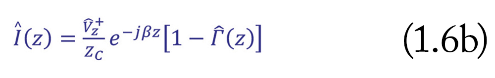
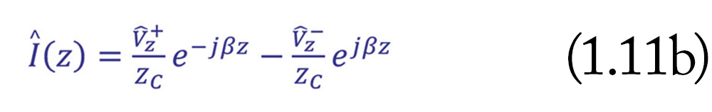
Equations (1.5b) and (1.6b) express voltage and current at any location z, away from the source, in terms of the unknown constant Vz+ and the voltage reflection coefficient Γ at any location z away from the source.
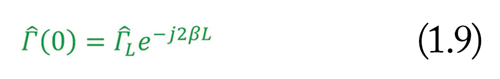
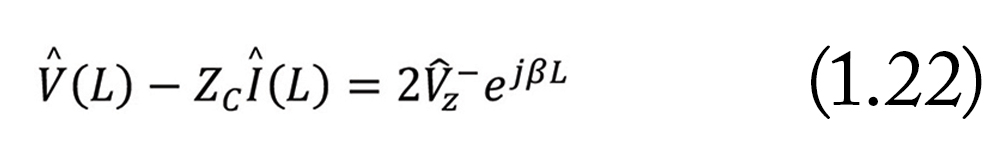
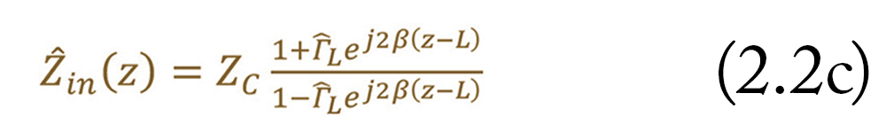
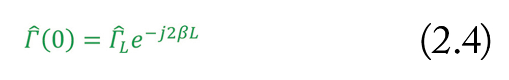
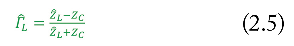
Let us return to this reflection coefficient, given by Eq. (1.3b). Letting z = L, we obtain the voltage reflection coefficient at the load
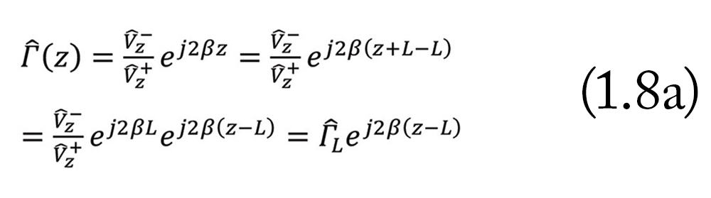
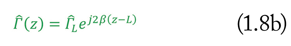
Thus, the voltage reflection coefficient at any location z, away from the source, can be expressed in terms of the load reflection coefficient as
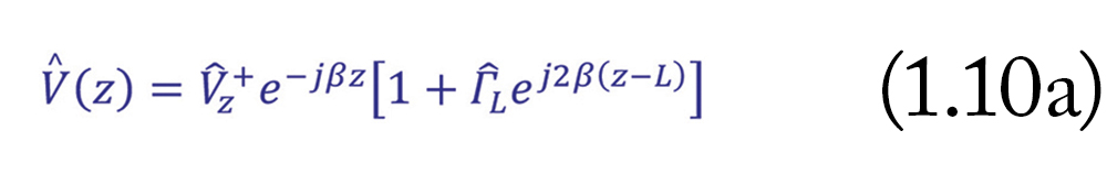
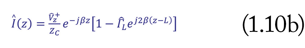
Equations (1.10) express voltage and current at any location z, away from the source, in terms of the unknown constant Vz+ , and the load reflection coefficient.
In summary, the voltage and current at any location z, away from the source, can be obtained from
or
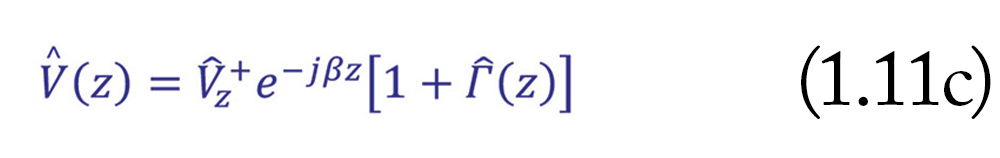
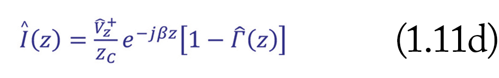
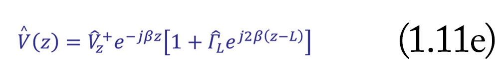

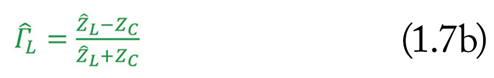
The last set of equations is perhaps the most convenient since the load reflection coefficient, ΓL, can be obtained directly from Eq. (1.7b) and the only unknown in this set is the constant Vz+.
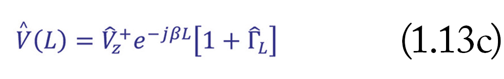
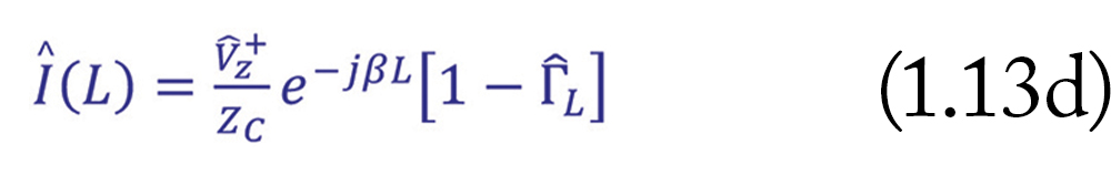
The three sets of equations (1.11) can be used to determine the voltage and current at the input to the line, and at the load.
Letting z = 0, in Eqns. (1.11) we obtain the voltage and current at the input to the line as
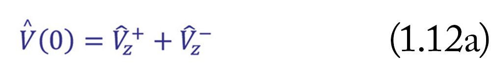
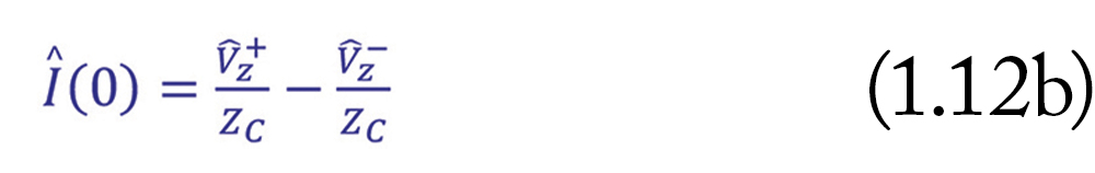
or
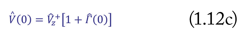
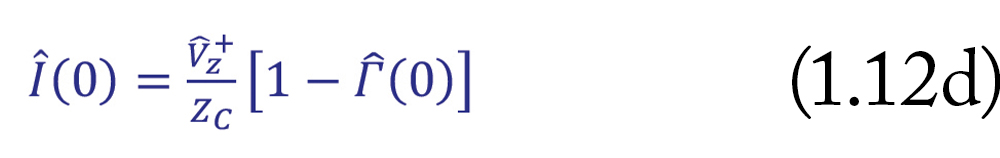
or
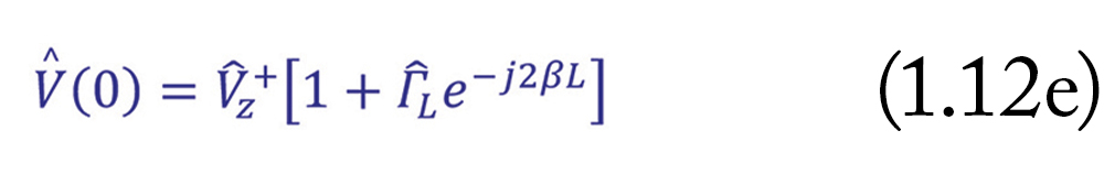
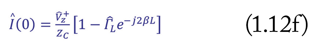
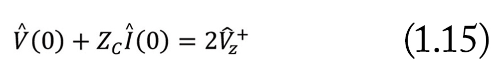
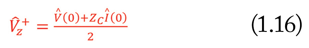
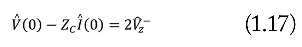
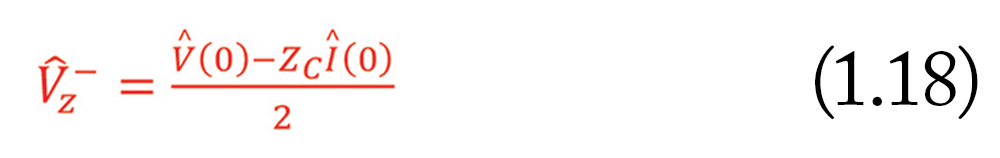
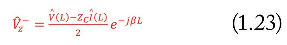
Next, let us turn our attention to the undetermined constants Vz+ and Vz–. These constants can be determined from the knowledge of the voltage and current at the input to the line.
Eqns. (1.12a) and (1.12b) can be rewritten as
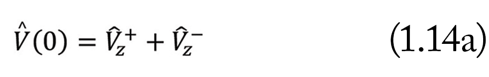
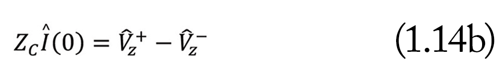
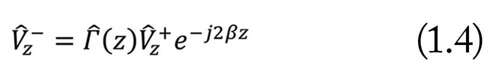
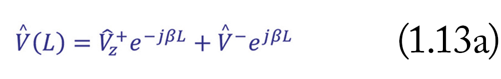
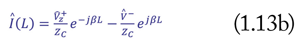
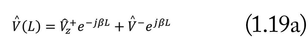
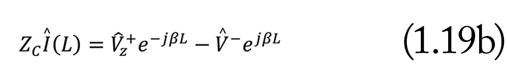
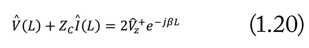
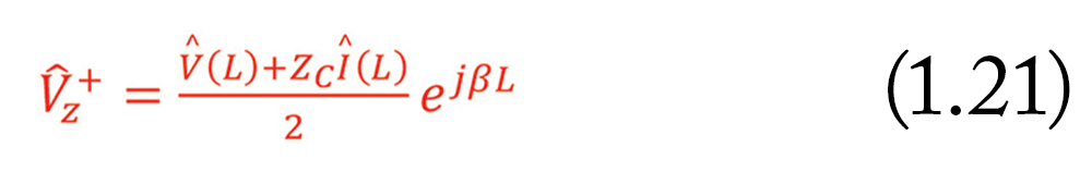
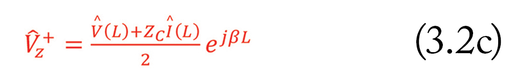
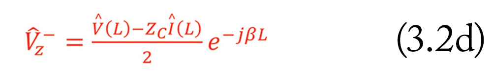
These two undetermined constants, Vz+ and Vz–, can alternatively be obtained from the knowledge of the voltage and current at the load.
Eqns. (1.13a) and (1.13b) can be rewritten as
Observation: To obtain the voltage or current at any location z, away from the source, we need the knowledge of the undetermined constants, Vz+ and Vz–, (or at least Vz+). To obtain the undetermined constant, Vz+ and Vz–, we need the knowledge of the voltage and current at the input to the line, or at the load. We resolve this stalemate by introducing the concept of the input impedance to the line.
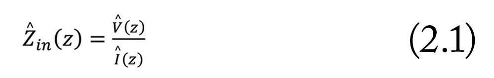
2. Input Impedance to the Line at any Location z away from the Source
At any location z, away from the source, the input impedance to the line, Zin, shown in Figure 2, is defined as the ratio of the total voltage to the total current at that point.
Since the total voltage and current at any location z away from the source can be obtained from the three different sets of Eqns. (1.11), it follows that the input impedance to the line, at any location z away from the source can be obtained from
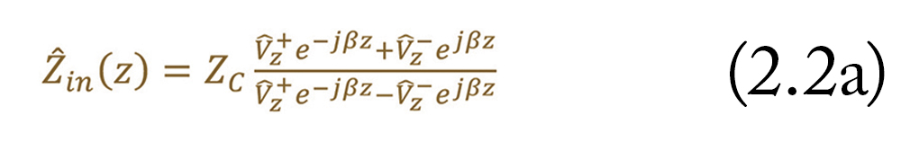
or
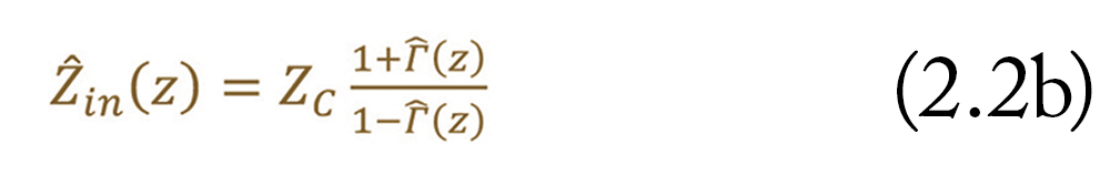
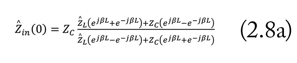
Letting z = 0, in Eqns. (2.2) we obtain the input impedance to the line at the input to the line as
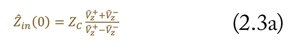
or
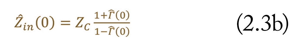
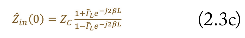
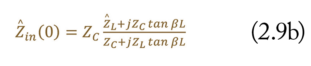
Since the constants, Vz+ and Vz–, are still unknown, in the calculations of the input impedance to the line at the input to the line, we are left with the remaining two equations, (2.3b) and (2.3c).
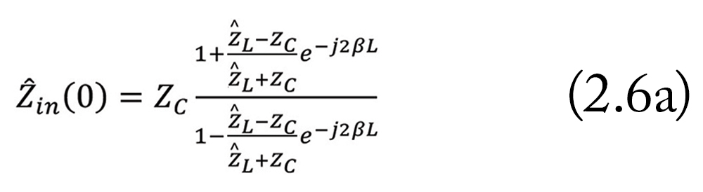
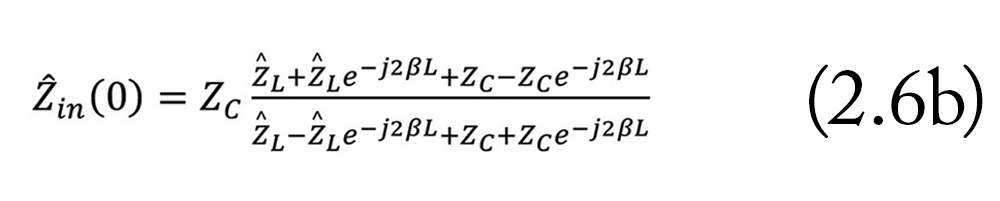
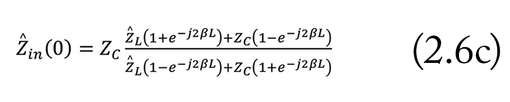
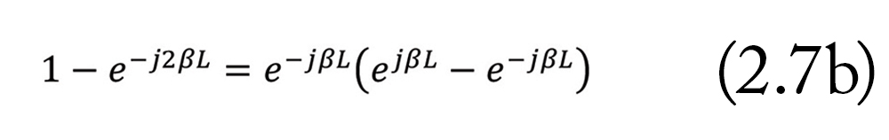
Since,
and then use Eq. (2.3c) or Eq. (2.9b), derived next, to calculate the input impedance to the line at the input to the line.
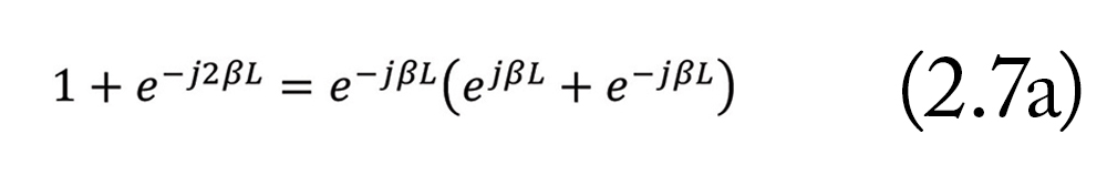
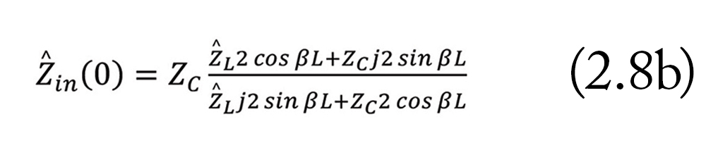
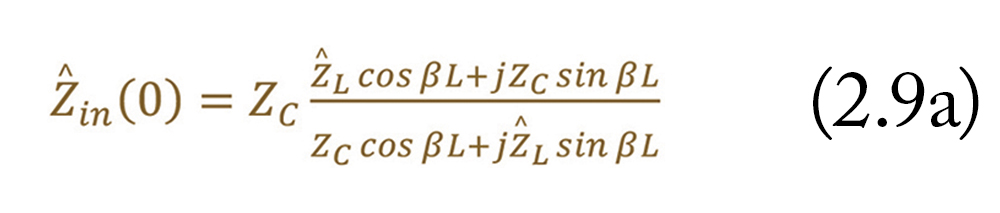
There is one more useful set of formulas for obtaining the input impedance to the line at the input to the line. Using Eq. (2.5) in Eq. (2.3c) we get
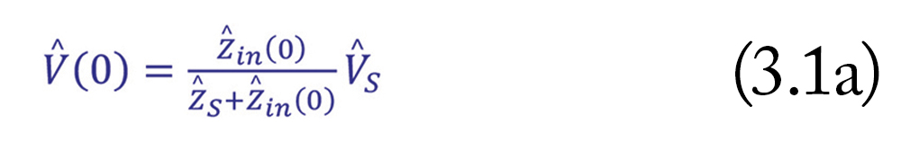
3. Voltage and Current at the Input to the Line
At the input to the line, we have a situation depicted in Figure 3.
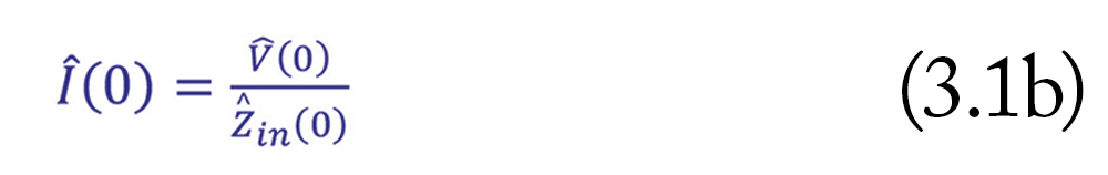
It is apparent the voltage and current at the input to the line can be now obtained from
Now, from the knowledge of V and I we can determine the constants Vz+ and Vz– from
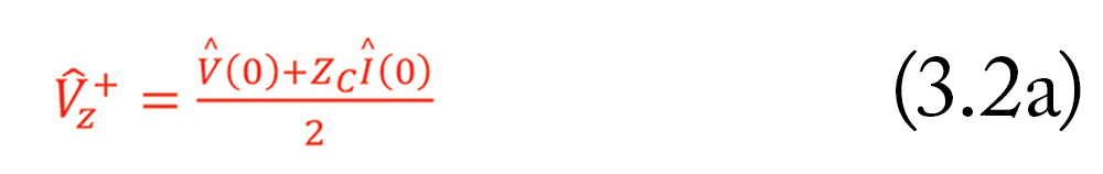
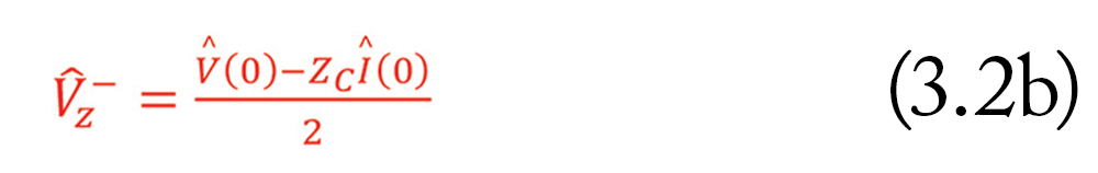
or
At this point we can obtain the voltage, current, or impedance at any location z away from the source using the previously derived equations.
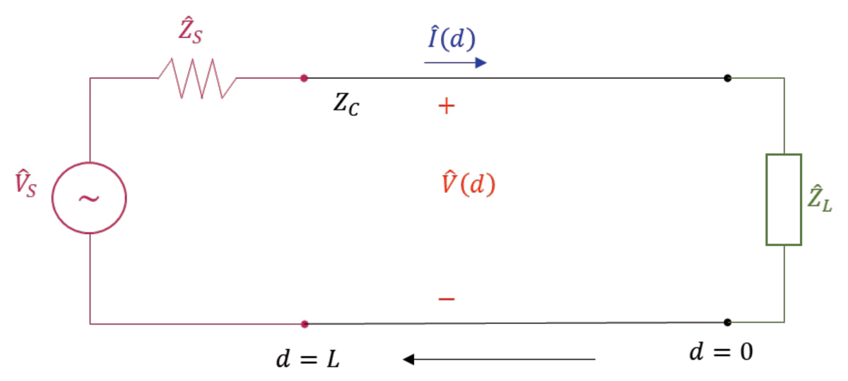
In the next article, we will analyze the circuit where we move from the load is located at d = 0 towards the source located at d = L (Model 2). Such a circuit is shown in Figure 4.
References
- Adamczyk, B., “Sinusoidal Steady State Analysis of Transmission Lines – Part I: Transmission Line Model, Equations and Their Solutions, and the Concept of the Input Impedance to the Line,” In Compliance Magazine, January 2023.
