Sinusoidal Steady State Analysis of Transmission Lines

EMC Concepts Explained

Part III: Voltage, Current, and Input Impedance Calculations – Circuit Model 2

his is the third of the three tutorial articles devoted to the frequency-domain analysis of a lossless transmission line. In the previous article, [1], several methods of calculating the voltage, current and input impedance along the lossless transmission line were presented, using Circuit Model 1, shown in Figure 1.

In this model, the source is located at z = 0, and the load is located at z = d. The voltage, current, and input impedance were derived as a function z, when moving from the source towards the load.

In this article, we will present the results for the voltage, current, and input impedance derived from the transmission line circuit shown in Figure 2, referred to as Circuit Model 2.

In this model, the load is located at d = 0, and the source is located at d = L. The voltage, current, and input impedance now are a function of d, when moving from the load towards the source. Note that the input impedance to the line at any location d, Z_in (d), is always calculated looking towards the load, regardless whether we use Model 1 or Model 2.

1. Voltage and Current at any Location d away from the Load

Figure 1: Model 1 – the source located at z = 0 and the load at z = L

Figure 2: Model 2 – the load located at d = 0 and the source at d = L

The two distance variables are related by

In [1] the voltage and current at any location z away from the source were derived as

Using the relations (1.1), the voltage and current at any location d away from the load are

leading to

where

The solutions in Eqns. (1.5) consist of the forward- and backward-traveling waves. The forward-traveling voltage wave is described by

while the backward-traveling voltage wave is given by

Using these two waves, we define the voltage reflection coefficient at any location d, as the ratio of the backward-propagating wave to the forward-propagating wave

Thus,

From Eq. (1.8b) we obtain

Utilizing Eq. (1.9) in Eq. (1.5a) gives

Utilizing Eq. (1.9) in Eq. (1.5b) gives

Equations (1.10b) and (1.11b) express voltage and current at any location d, away from the load, in terms of the unknown constant V_d+ and the voltage reflection coefficient Γ(d), at any location d away from the source.

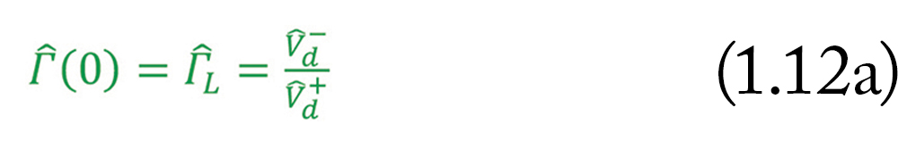
Let us return to this reflection coefficient, given by Eq. (1.8b). Letting d = 0, we obtain the voltage reflection coefficient at the load

Note that the load reflection coefficient can always be obtained directly from the knowledge of the load and the characteristic impedance of the line as

Utilizing Eq. (1.12a) in Eq. (1.8b) we get

Which expresses the voltage reflection coefficient at any location d, away from the load, in terms of the load reflection coefficient.

Equation (1.8b) can be used to determine the voltage reflection coefficient at the input to the line, i.e., at d = L, (we will need it shortly),

Utilizing Eq. (1.13) in Eqns. (1.10b) and (1.11b) gives

Equations (1.15) express voltage and current at any location d, away from the load, in terms of the unknown constant V_d+, and the load reflection coefficient.

In summary, the voltage and current at any location d, away from the load, can be obtained from

The last set of equations is perhaps the most convenient since the load reflection coefficient, Γ_L, can be obtained directly from Eq. (1.12b) and the only unknown in this set is the constant V_d+ .

Figure 3 compares the results for Model 2 to those of Model 1.

Figure 3: Model 1 vs. Model 2 – voltage and current along the line

The three sets of equations (1.16) can be used to determine the voltage and current at the load and at the input to the line.

Letting d = 0, in Eqns. (1.16a) and (1.16b) we obtain the voltage and current at the load as

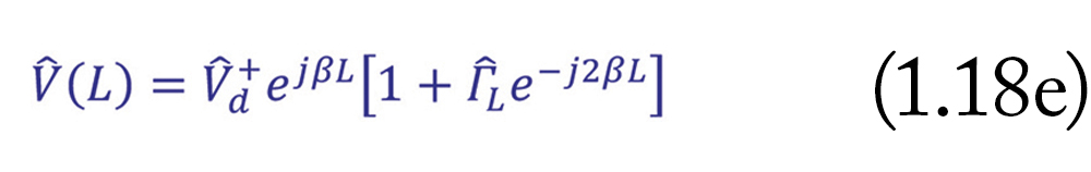
Letting d = L, in Eqns. (1.11) we obtain the voltage and current at the input to the line as

Next, let us turn our attention to the undetermined constants V_d+ and V_d–. These constants can be determined from the knowledge of the voltage and current at the load.

Eqns. (1.17a) and (1.17b) can be rewritten as

Adding Eqns. (1.19a) and (1.19b) gives

and thus

Subtracting Eq. (1.19b) from Eq. (1.19a) gives

and thus

These two undetermined constants V_d+ and V_d– can alternatively be obtained from the knowledge of the voltage and current at the input to the line.

Eqns. (1.18a) and (1.18b) can be rewritten as

Adding Eqns. (1.24a) and (1.24b) gives

and thus

Subtracting Eq. (1.24b) from Eq. (1.24a) gives

and thus

Observation: To obtain the voltage or current at any location d, away from the load, we need the knowledge of the undetermined constants V_d+ and V_d– (or at least V_d+). To obtain the undetermined constants V_d+ and V_d–, we need the knowledge of the voltage and current at the input to the line, or at the load. We resolve this stalemate in a similar way we did in [1], by introducing the concept of the input impedance to the line.

2. Input Impedance to the Line at any Location d away from the Load

At any location d, away from the source, the input impedance to the line, Z_in, shown in Figure 2, is defined as the ratio of the total voltage to the total current at that point.

Since the total voltage and current at any location d away from the source can be obtained from the three different sets of Eqns. (1.16), it follows that the input impedance to the line, at any location d away from the load can be obtained from

Figure 4 compares the results for Model 2 to those of Model 1.

Figure 4: Model 1 vs. Model 2: input impedance to the line

Letting d = L, in Eqns. (2.2) we obtain the input impedance to the line at the input to the line as

Since the constants V_d+ and V_d– are still unknown, in the calculations of the input impedance to the line at the input to the line, we are left with the remaining two equations, (2.3b) and (2.3c).

Since,

at this point, we effectively have just one equation (2.3c) to determine the input impedance to the line at the input to the line. Towards this end, we first determine the load reflection coefficient from

and then use Eq. (2.3c) or Eq. (2.7b), shown next, to calculate the input impedance to the line at the input to the line.

There is one more useful set of formulas for obtaining the input impedance to the line at the input to the line. Using Eq. (2.5) in Eq. (2.3c) we get

The right-hand-side of Eq. (2.6) is equivalent to, [2],

or equivalently,

3. Voltage, Current, and Input Impedance to the Line at any Location d away from the Load

At the input to the line, we have a situation depicted in Figure 5.

Figure 5: Equivalent circuit at the location d = L

It is apparent the voltage and current at the input to the line can be now obtained from

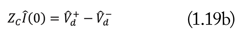
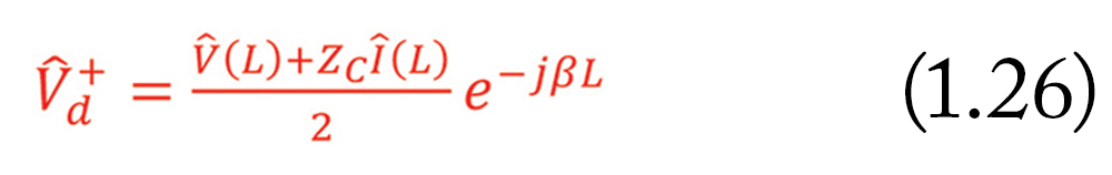
Now, from the knowledge of V(L) and I(L) we can determine the constants V_d+ and V_d– from

At this point we can obtain the voltage, current, or impedance at any location d away from the load using the previously derived equations.

References

Adamczyk, B., “Sinusoidal Steady State Analysis of Transmission Lines – Part II: Voltage, Current, and Input Impedance Calculations – Circuit Model 2,” In Compliance Magazine, February 2023.

Share this story:

Dr. Bogdan Adamczyk is professor and director of the EMC Center at Grand Valley State University (http://www.gvsu.edu/emccenter) where he regularly teaches EMC certificate courses for industry. He is an iNARTE certified EMC Master Design Engineer. Prof. Adamczyk is the author of the textbook “Foundations of Electromagnetic Compatibility with Practical Applications” (Wiley, 2017) and the upcoming textbook “Principles of Electromagnetic Compatibility with Laboratory Exercises” (Wiley 2022). He can be reached at adamczyb@gvsu.edu.

Back to Issue