(Re)Discovering the Lost Science of Near-Field Measurements

Understanding Radiated Emissions Measurements Made at One-Meter Separation: It’s Not What You’ve Been Led to Believe

Background¹

The first article in this series (see “Seventy Years of Electromagnetic Interference Control in Planes, Trains, and Automobiles (and Ships and Spaceships, as well)”) described in detail the use of radios that used unshielded connections (termed antenna lead-ins) between the radio and the external antenna.² The antenna lead-in was a single wire above ground, using aircraft structure for a return path, that was connected to high impedances at both ends. That is, the radio input was the grid of a vacuum tube, so basically a small capacitance, and the external antenna was an electrically short wire over most of the 0.15 – 20 MHz (200 –15 meters) frequency (wavelength) range of the radio.

U.S. Naval Air Development Center report

NADC-EL-5515 is the Rosetta Stone of the EMC discipline

Figure 1 shows a WWII-era handbook drawing of such an installation.³ Handbooks of the time went to great lengths showing photographs of poor and good radio antenna lead-in installations.⁴ Controlling the loop area of the lead-in over ground relative to that of adjacent culprit noise emitters (crosstalk) was emphasized.

Diagram with typical installation of radio, antenna, and ground connections for a WWII-era

Figure 1: Typical installation of radio, antenna, and ground connections for a WWII-era 0.15 – 20 MHz radio installation.

The specification that introduced EMI requirements based on controlling interference to/from these unshielded transmission lines was MIL‑I‑6181B, released in May 1953.⁵ As described in Reference 2, a report is available describing the selection of test antennas and set-ups for measuring to limits controlling radiated coupling to the unshielded antenna lead-in.⁶ NADC‑EL‑5515, released in 1955, is the rationale behind the radiated emission measurement limits and test methods of MIL‑I‑6181B.

NADC‑EL‑5515 should be required reading for every vehicle EMC engineer. If the physics described in NADC‑EL‑5515 were universally understood by EMC engineers, there would be no need for the near field physics discussion in this article. Unfortunately, this knowledge is truly lost, and it is apparent from the state of aerospace (RTCA/DO-160 section 21) and automotive vehicle radiated emission EMI specifications (CISPR 25), and standards that support them (SAE ARP-958), that such understanding is sadly lacking.^7,8,9

Purpose

Hence, the true purpose of this article, which is only peripherally historical. The reader is requested to be patient, as much of what is presented will appear at first rather obvious. The more obvious, the better, because the conclusion is antithetical to most people’s thinking, and a surprising conclusion is much more convincing if the trail there is familiar and well-worn. The conclusion is this simple: only a far-field measurement results in a true field intensity measurement. That is, the signal level measured at the EMI receiver, adjusted for any losses/gains in the transmission line path, is only relatable to a specific field intensity when the antenna’s physical aperture is immersed in a field of constant amplitude across it.

Under any other conditions (the near field) that relationship cannot be made, and any artificial attempts (one-meter field intensity limits supported by a one-meter antenna factor) are not only doomed to failure but also wrongheaded. This means that there is no valid use for such artificial constructs, and they lead to bad engineering decisions. This is not to say that near-field measurements are useless – far from it. A near-field measurement is absolutely necessary when the actual culprit – victim interaction is near field. But the point is, far- vs. near-field measurements are not simply quantitatively, but also qualitatively different.

We will start by defining and differentiating the concepts of far and near fields, all from an EMI test point of view. Far field is easiest, so we begin there.

Far Field

The far field as an abstraction is a simple concept to visualize and understand intuitively. The near field is more complex, but as a starting point, we are in the near field when we are not in the far field. In terms of radiated emission measurements, the concept of far field is mostly associated with standards such as CISPR 22 and the newer 32.^10,11 These standards provide for test sample/antenna separations of 3 to 30 meters at and above 30 MHz. The far field assumption means limits scale directly with separation distance. It also means that – and this is key – these standards do not specify antenna types, only that they be calibrated in the far field. As we shall see, limit scaling with distance and the assumption that the same result may be obtained with any suitably calibrated antenna are hallmarks of a far-field measurement. Neither of these is true in the near field. And this is what MIL‑I‑6181B and NADC‑EL‑5515 first presented to the EMC world, and which remains true to the present day, albeit too few practicing EMC engineers appreciate it.

All of the following criteria need to be met in order to be in the far field of a transmitting source:

The far field is traveling electromagnetic energy. That means the far field propagates independently of the existence of the transmitting antenna once it is launched. The electric and magnetic field components of a traveling wave (Poynting’s theorem) are in contrast to the quasi-static and induction field components close to the antenna, which begin and end on antenna elements, and vanish when the antenna excitation is removed. An example of the independence of the traveling wave from its source is the light from a distant star reaching Earth. The star may in fact no longer exist, but the light it radiated away is still traveling through space. Closer to home, one necessary (but insufficient in and of itself) requirement for achieving the far field is being at or beyond the distance at which the amplitude of the traveling wave exceeds that of the quasi-static and induction components. Heinrich Hertz derived this criterion for an electrically short dipole.

A far-field traveling electromagnetic wave emanates from a point source. This means that the wave front has spherical curvature. This doesn’t mean that the radiating source is literally a point, which would yield not only spherical curvature but also spherical symmetry. It means the transmitting source is so far away from the observation point that it appears as a point; the distance from the observation point to any point on the transmit antenna is equal. This assumption is inherent in the derivation of the Hertzian short dipole field components.
The wave front is not only spherical but also plane. Meaning that the sphere’s radius of curvature is large enough that over the physical aperture of our receive antenna there is no variation in field intensity or power density. The spherical wave front approximating a plane wave is the source of expressions for the far field such as 2D²/λ.

Now for the distance from an observation point to any point along an extended structure to be equal, the observation point must be infinitely far away. Similarly, a plane surface may be described as the surface of a sphere of infinite radius. But none of that is very practical for daily use. Instead, we decide on how closely our spherical surface needs to approximate a plane surface, typically by positing a maximum phase difference between any two lines from the observation point to different portions of the transmitting source. Figure 2 shows this process specifying the allowable variation from a plane wave as a fraction of a wavelength.

Figure 2: Geometry for determination of far-field distance based on how close a spherical wave front approximates a plane surface

In Figure 2, the circular arc struck between the radius labeled R and the radius that is its hypotenuse marks off the length of the hypotenuse that is greater than R and denotes it as a fraction of a wavelength. The value we assign to “a” depends on the application of interest.

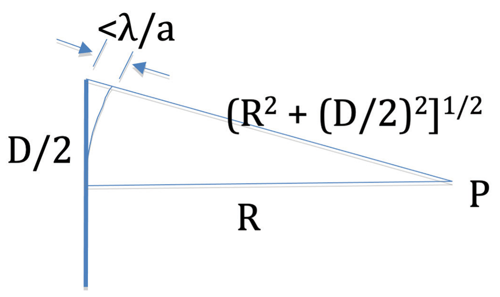
Setting
R + λ/a = √(R² + (D/2)²)

and solving for R, we get
R = (a/2λ) (D/2)² – λ/2a or
R = aD²/8λ – λ/2a

When we pick a maximum phase front variation of a sixteenth wavelength (a = 16), we get
R = 2D²/λ –λ/32

In order for this to approximate the familiar 2D²/λ, the first term must greatly exceed the second term. This is certainly the case when the transmit antenna is at least a half‑wavelength long.

From this analysis, in addition to learning/reviewing the derivation for 2D²/λ, we understand that it is based on a traveling electromagnetic wave far from the point source. We can also see that if the antenna is electrically short, the derivation doesn’t work at all. The phase difference between the two radial distances in Figure 2 will always be smaller than the phase difference associated with distance d/2. If the antenna dimensions are an insignificant fraction of a wavelength this problem formulation says the far field is at any distance from the antenna, including zero. That is, if the phase difference from the center of the antenna to its end is the same or smaller than the phase difference we posit as acceptable for the far field criterion, then even a point on the antenna centerline is in the far field in terms of the above analysis. This merely emphasizes that the analysis assumes an electrically long antenna and a traveling electromagnetic wave.

Near Field

Now let’s look at the opposite situation: the one‑meter radiated emission measurements that are very similar between MIL‑STD-461, and RTCA/DO‑160 section 21 and CISPR 25.¹² In these standards, minimum lengths of cables vary from 1.5 m (CISPR 25) to 3.3 meters (RTCA/DO‑160). This means that the antenna separation from the radiating structure is much less than the length of the radiating structure.

Figure 3a demonstrates that the radiating structure is not a point source. Further, the dimensions of the antennas used below 1 GHz are on the order of the separation distance, so that the test antenna is not measuring a single, constant amplitude of field intensity over its physical aperture, but instead is integrating a complex variation of field intensity over its physical length. Figure 3b shows the radiation situation most people visualize when making antenna measurements. Figure 3c is similar to Figure 3a and in direct contrast to Figure 3b, showing the extreme near field. Figure 3c is an end view of the isometric view shown in Figure 3a, showing the electric field due to a wire over a ground plane.

Figure 3c emphasizes that antenna placement is critical. Placement of identical antenna types at various positions from A to C reveals that the received signal will be dependent on the orientation of field lines, which is strongly a function of the position close to the test sample. Inspection of two of the same type antennas with different lengths at position D emphasizes that the longer antenna is not measuring constant field intensity over its physical aperture, but instead is integrating a variation of field intensity over its physical length. We cannot predict from the position D measurement with the smaller antenna what the larger antenna would measure because while the smaller antenna is illuminated by a near-constant amplitude electric field, the larger antenna is not. And we cannot extrapolate from the measurement with the larger antenna to using the same antenna or another antenna at another position, for the same reason.

In Figure 3b, the voltage measured at the antenna port where the phase front is constant over the antenna physical length is directly proportional to the field intensity impinging upon it. In contrast, in Figure 3c the single value of “field strength” derived from the voltage at the antenna is only representative of what is measured at this particular position relative to the test sample, and using a particular antenna, at a particular orientation. The measured value is not a scalable far field “field intensity” in the sense that one can use it to predict the field intensity at some other distance or measured with a different antenna.

Diagram showing antenna physical aperture for testing

Figure 3a: One-meter separation radiated measurements are near-field measurements. The test set-up boundary is longer than the distance to the measurement antenna. The antenna physical aperture (length in the case of the biconical) is of the same order of magnitude as the separation from the test sample. For the test set-up to be in the far field of the antenna, line segments AB and A’B would need to be approximately equal in length. Likewise, for the antenna to be in the far field of the test set-up, line segments A’B and A’B’ would need to be nearly equal in length. In a one-meter separation measurement, neither condition is obtained.

Figure 3b: The spherical wave front of a point source radiator. As the distance from the source increases, the spherical wave front appears increasingly planar. But planar is a relative quantity. The dimensions of the receive antenna also determine the far field distance. When the wave front is plane enough, measurements using different antennas will correlate.

Figure 3c: The electric field (red) of a wire suspended over a ground plane (orange). Field lines below the ground plane are images. Field lines to the right of the ground plane’s end point are not accurately rendered. They would curve around and connect at right angles to the ground plane. Wave front or field curvature is far from the plane, and correlation to another measurement at another distance using a different or even similar antenna is impossible.

A real-world example of these limitations is FCC rules for EMI testing on an open area test site (OATS) back in the 1980s. The original test method used half-wave dipoles at a three-meter separation from the test sample. At 30 MHz, this placed a 5-meter-long antenna at 3 meters distance. The antenna was longer than the separation: near field. When biconicals started to become popular as tunable dipole replacements, the FCC ruled that while biconicals were acceptable, if there were any question about whether the test sample met the limit, a dipole measurement would be made, and that result would be used. The ~140 cm biconical was actually a better far-field measurement due to its much shorter length, but the point was that a standard had to be maintained, and they knew that biconical and 30 MHz half-wave dipole measurements would not agree.

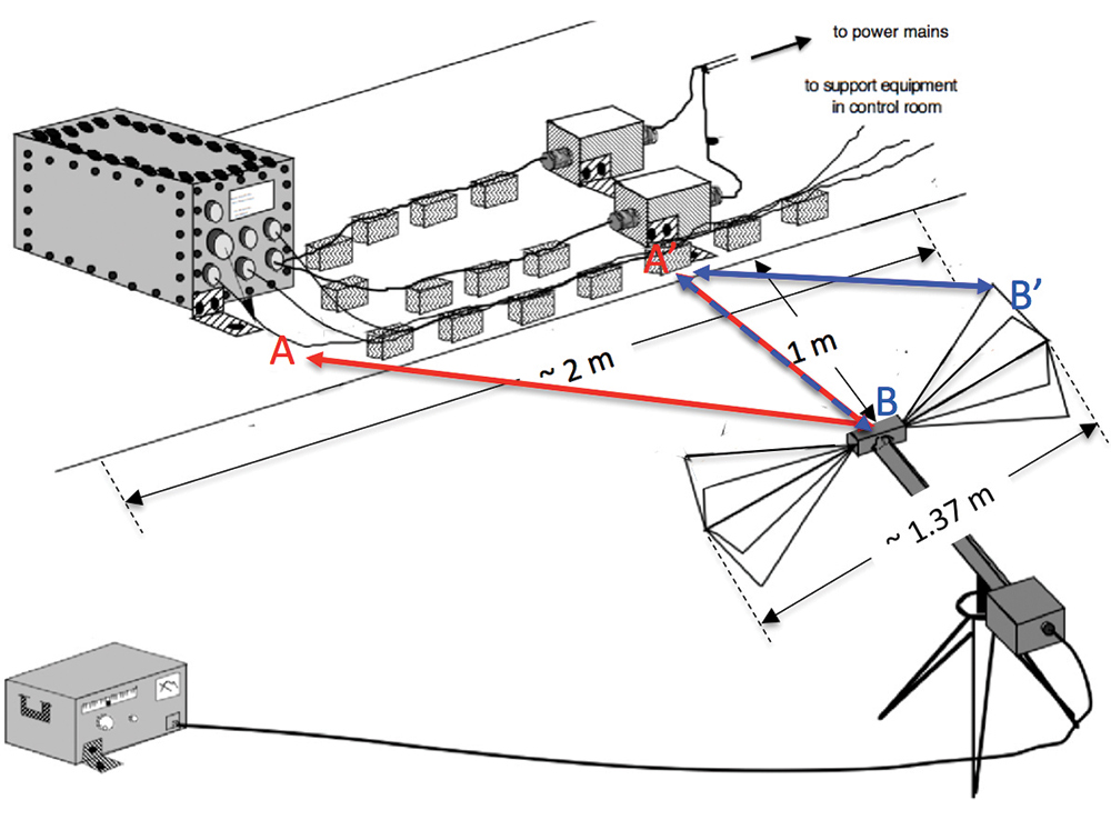
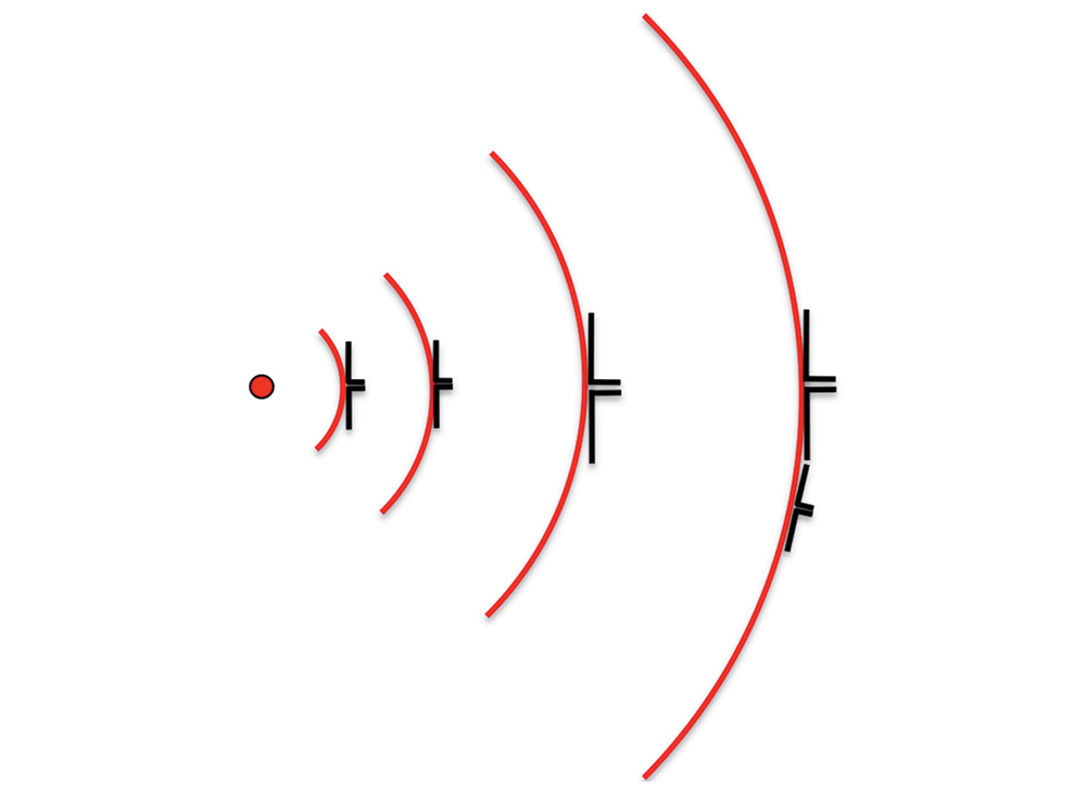
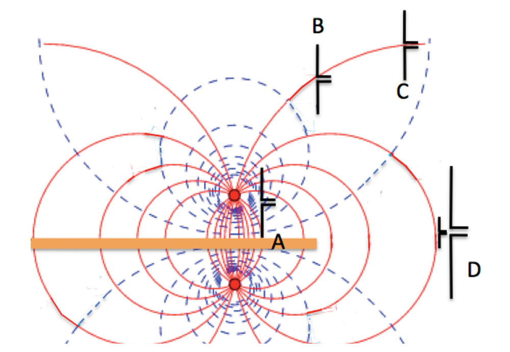
A final note about Figures 3a, 3b, and 3c: The issues illustrated are frequency independent. Regardless of frequency – dc to light – if the above conditions apply, the measurement is near field.

In the words of NADC‑EL‑5515, referring to antenna types used for EMI testing in the 1950s:

“For instance, a resonant dipole antenna has good sensitivity to low-impedance (magnetic) fields near its center and high-impedance (electric) fields near its ends. Other antennas, such as the discone, have a completely different distribution of impedance, polarization, physical size, and contour. Obviously, a comparison of the effect of a given interference field upon the dipole and the same field on a discone can only be made in a very general manner. For this reason, (MIL‑I‑6181B) radio interference limits are derived expressly for each particular antenna that is to be used, and an exact correlation between different types of antennas is not expected.”¹³

Near and Far Field Limit Derivation

It is instructive to compare and contrast how the limits in standards such as CISPR 22/32 were determined, vs. those in MIL-I-6181. Limit derivation for standards like CISPR 22/32 comes directly from specifications on the quality of radio services.¹⁴

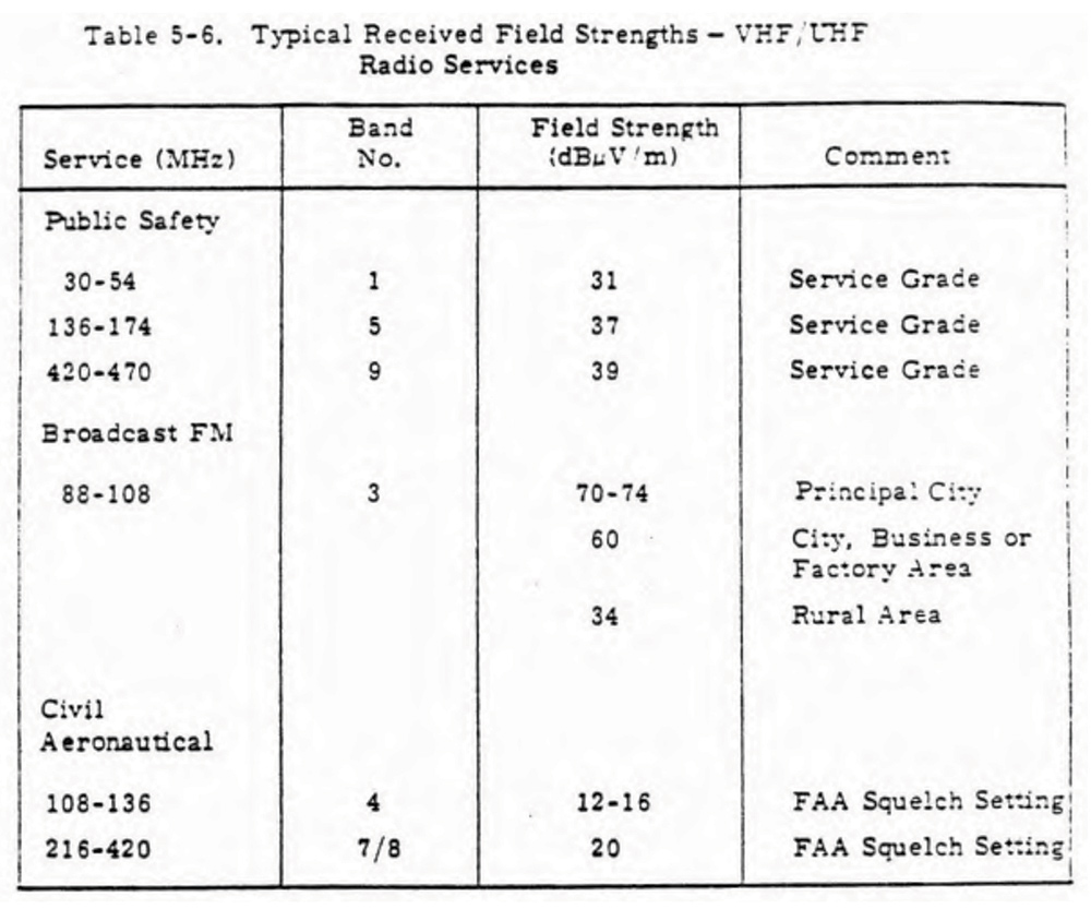
Figure 4 is an example excerpted from Reference 14. Such specifications state that a certain quality of baseband signal results when a specified level of broadcast signal is received. From this level, an EMI limit may be counted down using the signal-to-noise ratio required to get the specified baseband quality. Thus, it is completely natural to specify limits protecting such services in terms of field intensity, especially when the compliance measurement is made in the far field (or nearly so).

Table displaying published expected signal levels for various broadcast radio services

Figure 4: Published expected signal levels for various broadcast radio services (from Reference 14)

But the limits in MIL-I-6181B were not determined that way at all, and the success criterion for vehicle EMC is also not so determined. NADC-EL-5515 describes how the MIL-I-6181B limits were obtained, and this limit-setting exercise also determined the test method:

“These limits were decided upon as a result of tests made on a BC-384Q receiver installed in a shielded room. A 24-inch lead-in and a 12-foot straight wire antenna outside the shielded room were used to simulate an aircraft set-up. Various types of radio interference sources such as d-c motors, poorly shielded dynamotor cables, an adjustable output ignition source, etc., were installed at a distance of one foot from the lead-in. At those frequencies where interference sources happened to produce an interference signal which was slightly above the background of the BC-348Q, a measurement was made with an AN/PRM-1 in conjunction with its rod antenna. The rod was located one foot from the noise source, and the resultant measurement was taken as an approximation of the desired radio interference limit.”

Figure 5 is a recreation of the described limit setting measurement, based on the above passage. Two key points immediately suggest the vast difference from the CISPR 22/32 limit derivation. The first is this is entirely empirical, as opposed to using established specifications as a benchmark. The second is that the measurement distance is extremely near field, and the limits are in terms of the induced noise in the victims – no field intensities involved. When noise above the background is detected from the speaker connected to the radio’s audio output, the measured level at the AN/PRM-1 is recorded. The AN/PRM-1-meter displays microvolts and decibels above a microvolt. There is no antenna factor involved here. This is termed an antenna-induced limit and is a key concept that has been largely lost but is every bit as pertinent today as it was in 1953. Figure 6 shows MIL‑I‑6181B antenna-induced radiated emission limits.

Figure 5: Reenactment of MIL-I-6181B radiated emission limit setting procedure in the EMC Compliance screened test chamber

Figure 6: Figure 6a (41” rod) and Figure 6b (resonant dipole) antenna-induced radiated emission limits from NADC-EL-5515

Rigorously, “antenna-induced” means the theoretical open-circuit voltage that would appear at the antenna terminals with an electric field impinging upon it. Losses associated with any circuitry necessary to adapt from that open-circuit potential to a signal that can be piped down a transmission line must be accounted for. So, with the 41” rod antenna used as in Figure 5, there is no data reduction necessary: the receiver meter reading (plus any attenuation selected) is the reading to be compared to the limit.

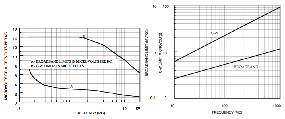
But above 30 MHz, where half-wave dipoles are employed, balun losses must be factored in, and NADC‑EL-5515 explains how to do that. In the days of antenna-induced limits, the loss associated with a matching network was termed the antenna factor. But unlike modern practice, the antenna-induced antenna factor is a unit-less loss factor (dB), whereas the modern antenna factor, being the inverse of antenna effective height, has units of meter^-1, or dB per meter.

Of course, any cable losses must be accounted for as well, just as in a field intensity measurement. The concept of an antenna-induced limit may seem foreign, but there is a close modern example with which an EMC engineer should be familiar. Radiated emission measurements such as those described above are designed to force good EMC design at the equipment level, so that at system or platform integration, there are no ugly surprises resulting in delays or costly modifications at the last minute. The “proof of the pudding” is verification that all platform antenna-connected receivers can operate interference-free.

With such receivers often being tunable over thousands of channels, it is impractical to tune to and check each frequency. Instead, standards such as MIL-STD-464 mandate a “spectrum analyzer noise floor survey.”¹⁵ The transmission line connecting the receiver’s antenna is disconnected from the receiver, and instead attached to a spectrum analyzer or EMI receiver, which is set to sweep over the entire tunable range of the receiver, or multiple sub-bands if that is necessary. Signals appearing above the substituted receiver’s noise floor or some other level are then checked to see if they actually cause interference.

Figure 7: Compliance Design biconical antennas covering 30 MHz to 1 GHz (no longer manufactured). Frequency ranges shown are approximate. Smaller biconicals have identical elements, but different baluns. Photo courtesy of Glen Dash Foundation.

This is almost an antenna-induced measurement. The pass/fail criterion is a dBuV or more likely dBm level based on the particular receiver’s performance specification. A similar example may be found in the C & D revisions of MIL-STD-464, where antenna-induced measurements at a distance of one meter from Army ground vehicles are made using not EMI test antennas as in MIL-STD-461, but rather antennas representative of those next to which the ground vehicle might be parked (typically whips). The whips are connected to a spectrum analyzer, and the limit is again in terms of the rf potential or power at the connected spectrum analyzer.

The reader should be able to appreciate the high degree of similarity between these modern measurements and those described in NADC-EL-5515. The only difference is that the noise floor measurement is referenced to the receiver’s antenna input, so the matching of the antenna to the transmission line and any line losses are part of the answer and for which separate accounting is unnecessary.

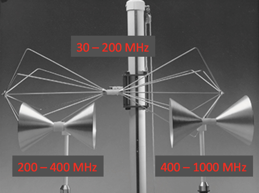
One other important facet of antenna-induced limits and the passages from NADC-EL-5515 is worth mentioning here. NADC-EL-5515 went to some length to explain the selection of antennas used for MIL-I-6181B 12” measurements. They were supposed to simulate the coupling to platform antenna-connected conductors (open-wire transmission lines). If one looks at antennas used beyond the biconical frequency range in vehicle EMI testing today, one finds horns and log-periodic arrays. The simulation of platform antennas for a good quality radiated emission test uses antennas with dipole‑like patterns, because such are either used on platforms, or in the case of high gain platform antennas, noise sources are typically in the back or at most side lobes of such, and thus are coupling via a low gain mechanism.

It is the author’s belief that biconical antennas such as the Compliance Design collection shown in Figure 7 would serve admirably. Even if antenna-induced limits were not invoked, it is the author’s opinion that such antennas are superior to what is used today above 200 MHz. With an antenna-induced limit, one could compare the output of the Figure 7 antennas to what would be required at a platform-level spectrum analyzer survey. Even without an antenna-induced limit, given the similarity between the EMI test and platform-installed antennas, one could do the comparison to get a much better prognostication of the actual EMC “proof-of-the-pudding” test results.

The Switch From Antenna-Induced to Field Intensity EMI Limits

MIL-I-6181B instituted antenna-induced limits measured at 12” from the test sample and attached cables. NADC-EL-5515 explains why, and that MIL-I-6181B also prohibited the future procurement of receivers requiring the unshielded high-impedance lead-ins. This means the stringent limits applied at 12” from the test sample were a grandfather clause, protecting the current inventory of high input impedance installed radios until such time as they had all been replaced by more modern receivers designed to work with 50 Ω coaxial transmission lines. In the words of NADC-EL-5515:

“(MIL-I-6181B) requires that all equipment used with antennas be designed for use with a shielded antenna lead. If and when the unshielded antenna lead is completely eliminated from use in aircraft, a review of present methods and limits in the frequency range 0.15 to 20 mc will be required.”

With the prohibition of the unshielded transmission line, the radiated emission problem is greatly ameliorated. Instead of what amounts to a crosstalk control, coupling is now to an antenna, and antennas are mounted externally and are further removed from most noise sources than the transmission line between the antenna and the antenna-connected receiver.

When the Tri-Service Committee convened circa 1966 to fashion MIL-STD-461/2/3 out of the various Service and platform-unique EMI specifications, they apparently deemed it time to abandon the 12” grandfather clause. Army and Navy EMI specifications of the time were already making some radiated emission measurements at distances greater than one foot, and the one-meter separation that resulted may have been nothing more than a “metricized” average of the Army (5’ minimum), Navy (3’) and Air Force (1’) separations.^{16, 17, 18, 19}

MIL-STD-462 (1967) required the present one-meter separation between the test sample and the antenna.²⁰ With an antenna as the radiated emission victim, as opposed to a transmission line, it might have seemed natural to transition to a field strength type control. Whatever the reason, the move to a one-meter separation was accompanied by a shift to a field intensity limit, and the consequent need for the kinds of antenna factors we use today. Thus, SAE ARP-958 was published in 1968; one year after MIL-STD-462 was released.

For the record, it should be noted that forerunners to RTCA/DO-160 included antenna-induced radiated emission controls.^{21, 22} RTCA/DO-160 was first released in 1975, and by that time field intensity limits had superseded antenna-induced, as described. Automotive radiated emission practice was always field intensity control but that did not begin until the 1970s.

Practical Problems Arising from the Use of Field Intensity Limits in the Extreme Near Field²³

The term “extreme near field” has a specific quantitative meaning in this context. It means that the transmit-receive antenna separation is of the same magnitude as its physical aperture, or less. In the case of radiated emission measurements made one meter away from a test sample with 1.5 m or longer attached cables, not even the Hertzian dipole equations suffice to describe the near field. The Hertzian dipole field equations only apply when the separation distance is much larger than the radiating structure dimensions.²⁴

SAE ARP-958 uses the physical model of two identical antennas in each other’s far field (Friis equation) to calculate an “effective” gain at one-meter separation. This is an effective gain because the antennas are in each other’s extreme near field. Therefore, the antenna factor so derived is only valid for measuring the field at that distance, and the standard of value is that antenna’s response to its own field at that distance. There is no particular value to comparing the “field intensity” measured by (for example) a biconical to the field intensity that biconical would see from another biconical a meter away. In fact, it is quite harmful in that there is an unspoken (and incorrect) assumption on the part of many EMC engineers that the field intensity measured at one-meter separation is scalable in some prescribed manner so as to be able to predict what the measured field intensity would be at another distance.

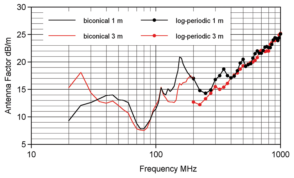
Figure 8 presents data gleaned from an old EMCO catalog. The same sort of information may be found on the ETS‑Lindgren website antenna page.25 If one-meter “field intensity” measurements were scalable, the antenna factors would be identical. Now proponents of field intensity measurements and one-meter antenna factors will rebut the use of such data, saying that one- and three-meter antenna factors are measured differently. And this is true, but it is not fundamental.

What is fundamental is that the assumption that extreme near-field intensity measurements are scalable violates one of the most fundamental laws of physics, namely the conservation of energy or power.

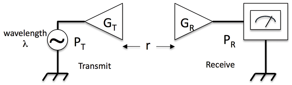
Based on the diagram of Figure 9, the Friis equation may be written as:

P_R/P_T = G_T G_Rλ² / (4πr)²

Chart displaying one- and three-meter antenna factors

Figure 8: One- and three-meter antenna factors

Diagram depicting set-up for understanding Friis equation

Figure 9: Set-up for understanding Friis equation

The Friis equation assumes that the separation distance places the antennas in the far field. In that asymptotic condition, the gain values are independent of separation, which is what makes far-field antenna calibration useful. But two elementary observations are apparent:

The left-hand side ratio is bounded by unity, and in practice will always be less than unity, or 0 dB; and

The right-hand side increases without bound as the separation decreases unless the gain values decrease commensurately.

The inescapable conclusion is that in close, gain is in fact a function of antenna separation. While gain or antenna factor asymptotically approaches a fixed far field value, this means nothing when the antennas are closer in than that.

Assuming half-wave dipoles (far field gain = 1.64 numeric, 2.15 dBi), one may solve the Friis equation for the distance at which the left-hand side ratio is unity, or 0 dB.

r = 0.13λ, or
r = D/4
where D is the half-wave dipole length

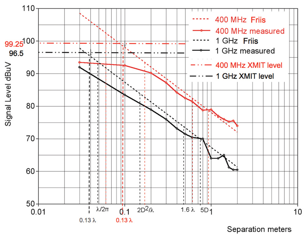
This is a purely theoretical construct that just says the gain must roll off at closer separations than this. Of course, the gain begins to roll off well before this calculated separation. The measured received power levels plotted in Figure 10 were taken using the set‑up of Figure 9, with separation “r” variable between 2 meters and 30 cm. Two different frequencies were evaluated: 400 MHz (λ = 75 cm, D = 37.5 cm) and 1 GHz (λ = 30 cm, D = 15 cm). Figure 10 shows measured vs. theoretical far field P_R/P_T ratios as a function of separation distance and wavelength. An inspection of Figure 10 shows that long before the far field calculation of received power shows it equal to transmit power, the response has rolled off.

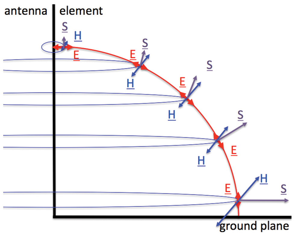
There are complicating factors involved in the close placement of two wire-type antennas, which include dipoles and biconicals. In very close proximity, there is capacitive coupling with which to contend and, above a ground plane, inductive coupling. Further, the direction of energy flow away from the antenna is different close to the antenna than farther away. Schelkunoff and Friis pointed this out long ago.²⁶ Figure 11a is copied from Reference 26 and shows the direction of energy flow (Poynting vector) away from the antenna element as a function of distance along the quarter-wave long antenna element itself and as a function of distance from the antenna. While the mathematics behind Figure 11a are complex, the notional Figure 11b drawing of the electric and magnetic fields from such an antenna provides an intuitive grasp.

The exact same effect is seen with higher gain antennas: gain derates rapidly from the far field values at separations less than a tenth of the far field distance (2D²/λ).²⁷ Figure 12 is copied from Reference 27 and shows gain derating for both dish and horn aperture-type antennas. Figure 12 is used in the following manner.

Chart displaying ratio of received vs. transmit power vs. half-wave dipole separation comparing the Friis equation and measured data

Figure 10: Ratio of received vs. transmit power vs. half-wave dipole separation comparing the Friis equation and measured data

Graph depicting Poynting vector direction as a function of position along the antenna and distance from the antenna

Figure 11a: Poynting vector direction as a function of position along the antenna and distance from the antenna. The solid lines are for an antenna element with a practical length-to-diameter ratio. The dashed lines are for a theoretical antenna element of vanishing diameter. (Reference 26, page 124)

Figure 11b: The ordinate axis represents a quarter wave stub over the abscissa ground plane. Electric field lines are constrained to be at right angles to a perfect conductor. The orientation of the electric field and the circulating magnetic field sets up the Poynting vector direction, as shown in the direction of the two axes. Note that the current vanishes at the tip of the quarter-wave stub, so no current means the Poynting vector amplitude vanishes, as well.

Figure 12: Fresnel zone power density from high gain aperture-type antennas normalized to the power density obtained at the far field boundary (copied from Reference 27).

Power density or equivalent field intensity is calculated using the far field gain at the 2D²/λ far-field boundary. Then the appropriate curve is followed inward to the Fresnel zone distance of interest. Here there are no complicating near-field effects from capacitive or inductive coupling, and the quasi‑static and inductive regions are contained well within the antenna feed point or phase center. They do not propagate down the waveguide to reach the antenna aperture itself.

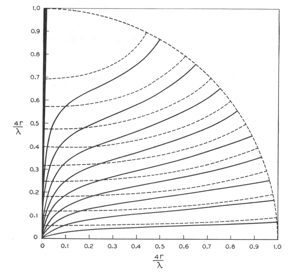
The Reference 27 handbook citation is not the origin for this work. It goes back over sixty years and is hardly new.²⁸

Theoretical Problems Resulting from Using Field Intensity Limits Where Antenna-Induced Is More Appropriate

Ignorance of the fundamentals of extreme near field measurements and of gain derating and the nature of the Fresnel zone has pronounced and dangerous impacts on both EMI and EMC requirements and verification. The following sections provide some relevant case histories.

Conflating Radiated Emissions and Radiated Susceptibility

With radiated emission and radiated susceptibility requirements both having field intensity limits, the idea that radiated emission (RE) and radiated susceptibility (RS) control were somehow two sides of the same coin became prevalent. People claiming that one controls RE to avoid RS was enough of a problem that in 1993 instructions were included in MIL-STD‑461D specifically saying that this belief is not true and that, in fact, RE limits protect antenna-connected receivers and RS limits provide a level of immunity to intentionally generated RF fields from high-power RF transmitters. These instructions have remained in all subsequent revisions of the standard.

Although the RE/RS comparison is extremely damaging, it is still assumed to be true by many engineers, often in the space community.²⁹ It is easy to see why: the space community doesn’t typically use the rf spectrum below several hundred megahertz, so there is no need for RE limits at lower frequencies, and often no or rudimentary RS limits there. Since they have used military limits covering as low as 10 kHz without comprehending the real need for such, they substitute this incorrect duality to justify using incorrect requirements. This leads to two errors. One is complete disrespect for the discipline, since comparing stringent RE limits to even the most rudimentary RS limits shows “margins” on the order of 100 dB.

The second error is to attempt to show the “margins” aren’t that high because a culprit (unintentional) emitter source may be placed very close to an (unintentional) victim receiver, requiring “scaling” of the one-meter RE limit to a distance of just a few centimeters. Such “scaling“ is done using Hertzian dipole field intensity behavior vs. distance, typically third order (cube of distance ratio).³⁰ Such comparisons are not accurate in the extreme near field, since the Hertzian dipole derivation assumes the observation distance is large with respect to the radiating structure dimensions – clearly not the case a meter away from a two-meter-long test sample.

While Hertzian dipole equations are often applied to various EMC-related problems and analyses, it is not difficult to see that they are inapplicable or at best only partially applicable to one-meter radiated emission measurements. One need not wade through the several‑page derivation in Reference 30. The inapplicability is at the very beginning, where the expression for the magnetic vector potential is derived.³¹ The requirement that the distance to the observation point be large with respect to the dimensions of the radiating element is inherent in the Hertzian expression for the magnetic potential vector, from which the entire derivation proceeds. It should not be surprising that the Hertzian dipole field expressions all “blow up” close to the source. The simplifying assumption that the distance to the observation point is large with respect to the dimensions of the radiating element means that the radiating source is a point. If there is current (flow of charge) on a point source, charge separation and potential differences follow.

Reference 24 derives and shows that, in the direction of maximum radiation, the Hertzian expression for the electric field is off by 3 dB when the separation distance is twice the dipole length, and that the electric field in closer than that approaches a fixed level proportional to the charge separation divided by the dipole length. When the observation point separation is one-tenth the dipole length, the Hertzian expression is 60 dB too high.

Since 1993, MIL-STD-461 has included in the CE102 limit rationale the information that, in the rod antenna range, the relationship of the measured radiated field to the voltage on a 2.5-meter-long wire is such that the wire potential is 40 dB higher numerically than the radiated signal measured. Reference 32 provides analytical details.³² If the wire potential is 40 dB above the signal measured a meter away, and the wire is suspended 5 cm above the ground plane (-26 dB above one meter), that makes the field intensity between the wire and ground plane 66 dB higher than at one meter. That is an upper bound on such scaling.

A shorthand model for this is shown in Figure 4 in Reference 24. One end of the dipole is now a wire suspended 5 cm above the tabletop ground plane and its image below the ground plane is the other end, for a net dipole separation of 10 cm. Looking at the circled point on Figure 4 of Reference 24, the field falls off beyond 20 cm from the wire as the cube of the distance ratio. So, from 20‑cm to 1 meter away, the field falls off by a ratio of 5³, or 42 dB. From 20 cm away from the wire to the wire, the field intensity increases by about 20 dB. The ratio of the field intensity between the wire and the ground plane beneath it to the field intensity found at a point a meter away is 62 dB. That calculation is for a pair of separated charges. The answer is within a few dB of the exact calculation for a cable of significant extent, measured not at a point but using a 41” rod antenna. Not bad, and it serves to dispel the mistaken superstition that Hertz says things should blow up.

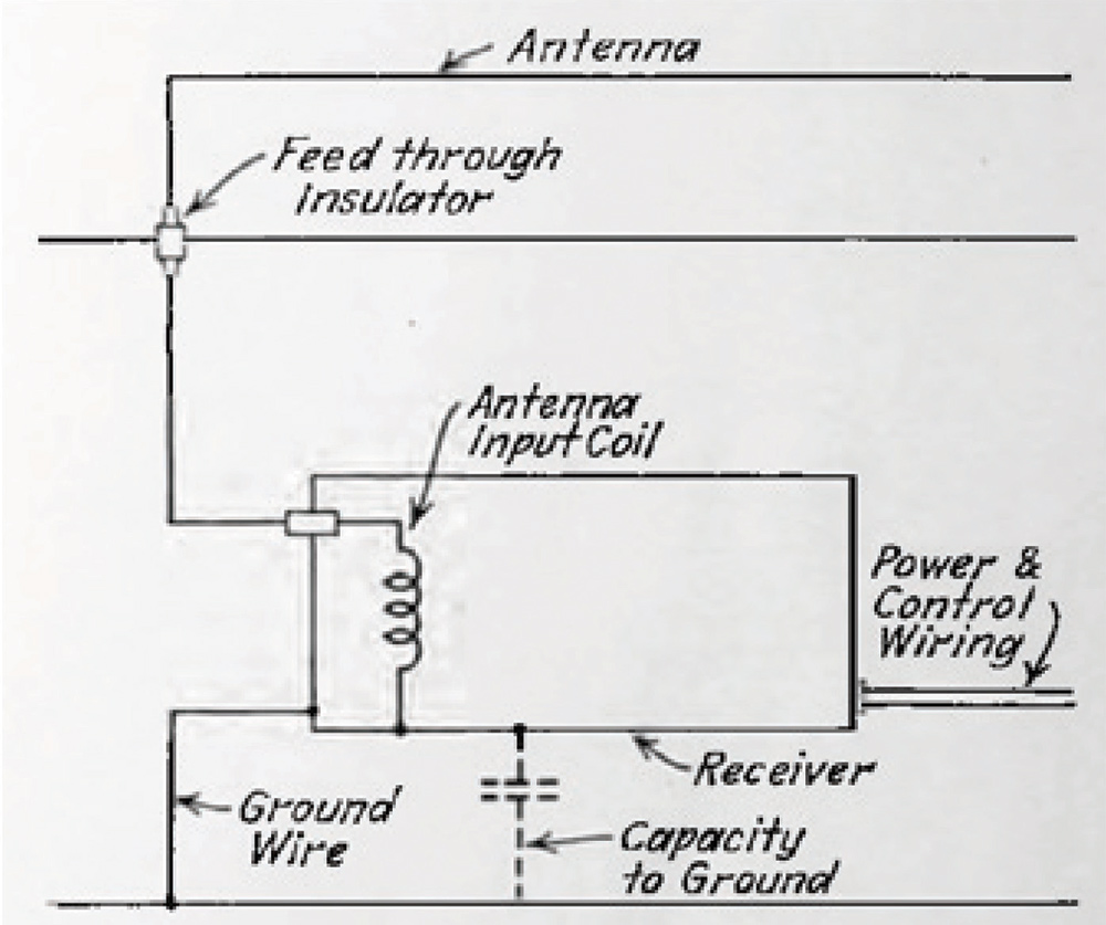
It should be noted that this is not about radiated energy at all. This is the fringing field from a source of charge separation. In this model, the only current that could contribute to actual radiation is the displacement current between the wire and the ground plane, and using a value such as 10 pF/m yields next to no current over most of the rod antenna frequency range. The fringing field dominates, and it dominates even more so at 12” than at a one-meter separation. Citing NADC-EL-5515:

“In general, the ratio of the electric to the magnetic components surrounding an unshielded lead will vary directly as the impedance of the load terminating the lead, and the apparent impedance presented to the various pick-up antennas will vary in the same manner. This statement applies to radial and tangential field components as contrasted with the more usual concept of wave impedance encountered in shielding theory, which applies only to the components tangential to the line of propagation.”

One-Meter Measurements Are Not Scalable Outwards, Either

Similar to the conflation misconception just described, people attempt scaling the one-meter results to a larger distance. Figure 13 portrays this type of an error. Some people advocate changing the one-meter measurements to three meters or more, based on the assumed accuracy superiority of far-field measurements. Some advocate for including the option of three-meter measurements in lieu of a one-meter measurement. The erroneous assumption is that one can adequately replace the other. As explained earlier, there are two errors here: 1) the radiation source is not a point source at either one- or three-meter distance; and 2) the one-meter measurement is not the field at some point in space but the average over the physical dimensions of the EMI test antenna. So not a scalable value in any way, shape, or form.

Cartoon strip of man looking for quarter he dropped in the wrong place

Figure 13: Controlling emissions at three meters or more for an interaction occurring at a one‑meter separation

Misapplying Antenna Factors

SAE ARP-958E (2021) now provides for separate horizontal and vertical polarization antenna factors for dipole-like antennas (dipoles, biconicals, log-periodic arrays). Under the right conditions this might make sense (given the a priori use of field intensity limits in the extreme near field) but it is indefensible given how they measure antenna factors.

The 1968 release SAE ARP-958 was for the newly mandated log spirals of MIL-STD-461.³³ SAE ARP‑958 did not specify the height of the antennas above the floor, nor even if the floor would be reflective or not. But SAE ARP-958A (1992) specified a reflective floor and a three-meter height above the floor.³⁴ The purpose was to control ground plane effects and make them negligible relative to the direct coupling between transmit and receive antennas. All subsequent revisions maintained the three-meter height and the reflective ground plane.

Note that, while all one-meter separation radiated emission requirements (CISPR 25, RTCA/DO‑160, and all revisions of MIL-STD-461/-462) place the antennas approximately one meter above the ground plane, SAE ARP-958E measures the separate polarization-based antenna factors three meters above the ground plane. Ground plane effects measured at three meter height are not even remotely applicable when antennas are one meter above the ground plane. Consider that over fifty years ago, just a few years after the biconical antenna was introduced in MIL-STD-461 (1967), a handbook warned that placing the lower tip of a vertically oriented biconical within two feet (61 cm) of the floor would capacitively load it sufficiently to change the antenna factor.³⁵

The point is this: if you want the biconical placed with the lower tip one foot above the floor (CISPR 25), then fine, make it so. And make everyone do it the same way. But then don’t apply a correction factor measured at three meters above the ground to correct for that. Don’t correct for it at all. Just mandate the proper antenna, and its separation and orientation, and then record antenna output, adjusted for balun and cable losses.

Misapplying Far-Field Gain in Computing Power Density

The EMC departments of two aerospace vehicle manufacturers refused to perform system-level EMC verifications that required the use of RF absorber panel emplacements around their respective platforms. They based their decisions on the belief that the computed RF power density from a platform high-gain microwave dish exceeded the absorber power rating. This was based on computing the power density using the far-field gain (only achieved beyond 50 meters distance) at a distance of two meters from the dish.

In reality, the actual power density based on Figure 12 was orders of magnitude less and much less than the absorber panel rating. Further, an elementary calculation of the area over which the far-field gain would concentrate the beam at a two-meter distance would have been a few centimeters on a side, which should have been a tip-off. Another tip-off would have been a Friis equation calculation showing more received power than transmitted using the far-field gain close in.

Basing RE Limits on the Far-Field Gain of a High‑Gain Dish

A non-US space agency levied a millimeter wave radiated emission limit based on the far-field gain of a high-gain dish. The resulting limit was such that it could not possibly be instrumented. The Fresnel-zone gain of such a dish at a one-meter distance is again orders of magnitude less than in the far field, plus the potential noise sources are in the back lobes of the antenna or, in a worst-case scenario, a 90-degree side lobe, but certainly not in the main beam.

Antennas Are Not Interchangeable in the Near Field

Both RTCA/DO-160, section 21, and CISPR 25 recommend but do not require the use of standardized antennas for radiated emission measurements. This is a direct consequence of using field intensity limits, and the assumption that the use of antenna factors is enough to yield the proper result no matter what antenna is chosen. The 1995 release of CISPR 25 went so far as to claim:

6.5.1 Antenna systems

“The limits … are listed in dB(uV/m), and thus theoretically any antenna can be used, provided that … the antenna correction factor is applied…”

This type of error was identified in 1967 when MIL‑STD-461 popularized the change from antenna-induced to field intensity limits.³⁶ The 2016 edition removes the egregious statement but only recommends standard antennas. In this regard, all versions of MIL-STD-461/-462 RE02/RE102 since 1967 are superior to RTCA/DO-160, section 21, and CISPR 25 in recognizing and accommodating the near-field nature of the measurement at a one-meter distance. The 41” rod antenna and 137 cm tip-to-tip length biconical have been required since 1967. From 1967 – 1993, log spirals were required from 200 MHz to 10 GHz. After 1993, the log spirals were replaced by double-ridge guide horns of specified aperture dimensions. Since 1993 the following rationale appendix wording explains the use of standardized antennas for requirement RE102:

“Specific antennas are required by this test procedure for standardization reasons. The intent is to obtain consistent results between different test facilities.

“In order for adequate signal levels to be available to drive the measurement receivers, physically large antennas are necessary. Due to shielded room measurements, the antennas are required to be relatively close to the EUT, and the radiated field is not uniform across the antenna aperture. For electric field measurements below several hundred megahertz, the antennas do not measure the true electric field.”

The first clause of the very last sentence is unnecessary since even if the calculated far field of the test antenna is no greater than one meter, the far field of the two‑meter‑long test set-up is clearly well beyond one meter. It is not enough for the transmitting source to be in the far field of the receive antenna; the receive antenna must also be in the far field of the source transmitter. Now it could certainly be the case that the transmitting source at microwave frequencies happened to be a small slot or aperture in the test sample enclosure, and if that were the sole radiating structure, it could be a far-field measurement. But the point is, one cannot know that a priori.

Shelf of electromagnetics books from Hertz onwards

Figure 14: A very small sampling of electromagnetics texts from Hertz onwards, in chronological order, with representation from every decade to one hundred years after Hertz (from the Museum of EMC Antiquities collection).

Conclusion

Converting near-field radiated emission control from field intensity to antenna-induced limits brings the following advantages:

Clear delineation between near-field vehicle and home/office/industrial plant far-field radiated emission controls;
Better correlation between equipment-level radiated emission limits and system-level EMC goals (direct correlation with spectrum analyzer noise floor surveys of platform antenna-connected receivers);

Diminution of wrong-headed EMC “engineering” comparing RE and RS controls as complementary functions; and
As a corollary, it would raise awareness of the real issues involved in RE control and improve the quality of EMC engineering, reducing episodes where bad science is used to justify programmatic decisions.

Even if a majority of the EMC discipline found these arguments persuasive, it would be wildly unrealistic to expect that over a half-century of tradition would be overturned. Given that reality, but with the understanding that antenna-induced is the ideal for one-meter radiated emission control, significant benefits could still result. The major such benefit would be dropping SAE ARP-958 altogether and using polarization-independent far-field antenna factors. Another possible advantage would be the adoption of EMI test antennas that better modeled those connected to platform-installed receivers that are the motivation for the levying of radiated emission controls.

And whether or not we return to antenna-induced near‑field limits, the discipline would benefit immensely if EMC engineers rediscovered the lost science of near‑field measurements. They could do worse than reading NADC-EL-5515. It also might not hurt to read Hertz’s original work on his dipole.

A WWII historian once remarked that other historians read books previous historians wrote, and then write a new book based on what they had read. In contrast, this historian always cited WWII-era sources. There is something to be said for original sources. The Museum of EMC Antiquities exists to preserve such knowledge and foster its study until such time that the present Dark Ages give way to an EMC Renaissance.

Illustration of Renaissance Era person writing

Endnotes

All standards and specifications referenced herein which are not copyrighted are available from http://www.emccompliance.com.
Javor, Ken, “Seventy Years of Electromagnetic Interference Control in Planes, Trains and Automobiles,” In Compliance Magazine, May 2023.
Also see Figures 2 and 3 of Reference 2.
NAVAER 16-5Q-517, Elimination of Radio Interference Problems in Aircraft, circa 1946-47.
MIL‑I‑6181B, Interference Limits, Tests and Design Requirements, Aircraft Electrical and Electronic Equipment, 29 May 1953.
NADC‑EL‑5515, Final Report, Evaluation of Radio Interference Pick-Up Devices and Explanation of the Methods and Limits of Specification No. MIL‑I‑6181B, 10 August 1955.
RTCA/DO-160, original through C revision, Environmental Conditions and Test Procedures for Airborne Equipment.
CISPR 25, all editions, various titles. “Limits and methods of measurement of radio disturbance characteristics for the protection of receivers used on board vehicles” is the 1995 title.
SAE ARP-958, all revisions, Broadband Electromagnetic Interference Measurement Antennas; Standard Calibration Requirements and Methods, 01 March 1968.
CISPR 22 – Information technology equipment – Radio disturbance characteristics – Limits and methods of measurement (withdrawn).
CISPR 32 – Electromagnetic Compatibility of multimedia equipment – Emission requirements.
MIL-STD-461E, and newer, Requirements for the Control of Electromagnetic Interference Characteristics of Subsystems and Equipment, 1999-present.
A discone antenna is half of a biconical, mounted vertically above or below a ground plane that provides the missing biconical element as an image in the ground plane.
CBEMA Report – CBEMA/ESC5/77/29 – “Limits and Methods of Measurement of Electromagnetic Emanations from Electronic Data Processing and Office Equipment,” 20 May 1977.
MIL-STD-464 and newer, Electromagnetic Environmental Effects Requirements for Systems, 1997 – present.
MIL-E-55301(EL), Electromagnetic Compatibility, 01 April 1965.
MIL-I-16910A(SHIPS), Interference Measurement, Radio, Methods, and Limits, 14 Kilocycles to 1000 Megacycles, 30 August 1954.
MIL-I-26600(USAF), Interference Control Requirements, Aeronautical Equipment, 02 June 1958.
The late Steve Caine was the chairman of the Tri‑Service Working Group that revised MIL‑STD‑461C (1986) and MIL-STD-462 (1967) into MIL‑STD-461D and MIL-STD-462D in the 1989 – 1993-time frame. He introduced the committee to the public at the 1989 IEEE EMC Symposium in Denver, saying that as he was the last surviving member of the original committee that fashioned MIL-STD-461/2/3 back in the ‘60s, it fell on him to lead the effort to clean up the mess they had made of it. When he was asked at another time about how some of the MIL-STD-461 limits and -462 test methods came about back in the ‘60s, he sighed and said, “Well, there was a lot of horse-trading going on back then.”
MIL-STD-462, Electromagnetic Interference Characteristics, Measurement of, 31 July 1967.
RTCA/DO-119, Interference to Aircraft Electronic Equipment from Devices Carried Aboard, 12 April 1963.
RTCA/DO-138, Environmental Conditions and Test Procedures for Airborne Electronic/Electrical Equipment and Instruments, 27 June 1968.
One prominent physicist refers to what the author terms the “extreme near field” as “inside the dipole.”
A complete mathematical treatment may be found in “Journey To The Center of The Dipole,” In Compliance Magazine, September 2023.
https://www.ets-lindgren.com/products/antennas?page=Products-Landing-Page
Schelkunoff, S.A. & Friis, H.T., Antennas, Theory and Practice, John Wiley & Sons, Inc. 1952.
NAWCAD TP 8347, Electronic Warfare and Radar Systems Handbook, October 2013
Hansen, R.C., and Bailin, L.L., “A New Method of Near Field Analysis,” IRE Transactions on Antennas and Propagation, December 1959.
Pearlston, C.B. Jr., “The Systems Approach in Designing a Specification for the Control of Radio Interference in an Airborne Environment,” Proceedings of the 5th Conference on Radio Interference Reduction and Electronic Compatibility. October 1959. In this work, Pearlston compares RE limits for protecting radio reception to susceptibility limits simulating rf transmitters, and while acknowledging the true purposes of each type of control, still manages to compare such limits and conclude that “100 dB” margins exist.
A complete derivation, leaving no “exercises for the reader,” is presented in Adamczyk, Bogdan, Foundations of Electromagnetic Compatibility with Practical Applications, John Wiley & Sons, 2017.
Javor, K. “Journey To The Center of The Dipole,” In Compliance Magazine, September 2023.
Javor, K., “On the Nature and Use of the 1.04 m Electric Field Probe,” ITEM 2011.
MIL-STD-461, Electromagnetic Interference Characteristics, Requirements for Equipment, 31 July 1967.
SAE ARP-958A, Electromagnetic Interference Measurement Antennas; Standard Calibration Method, November 1992.
White, Donald R. J., “EMI Test Instrumentation and Systems,” Volume 4, Section 3.3.4 of the Handbook Series on EMI & EMC, 1971.
Pearlston, C.B. Jr., Air Force Report No. SSD-TR-67-127, dated 1967. “Historical Analysis of Electromagnetic Interference Limits.” Pearlston makes the exact same points back at the inception that were presented in this article; these observations are hardly new:
“An academic argument could be made, and often has been, that “field intensity” is not a proper term to use in describing the phenomenon being measured and that “antenna-induced voltage” is much more descriptive of that phenomenon. Field intensity is generally defined as a measure of the intensity of the electric field; the term implies that the measured electric field gives a valid indication of the power density in the wave front, and permits an estimate to be made of the power coupled into a receiving antenna. Such an estimate is valid only in the far field where the plane wave phase relationships of electric and magnetic fields are fixed. Thus, the measurement does not give a valid indication of power coupling.

“Field intensity is also defined as the voltage induced in a conductor one meter long when held so that it lies in the direction of the electric field and at right angles to the direction of propagation and to the direction of the magnetic field. It can be argued that the equipment near-field does not have a uniphase front, and so the straight rod or dipole antenna will not necessarily be in the direction of the electric field. These near-field effects become even more marked at the higher frequencies where horn and parabolic reflectors are used.

“The term field intensity should refer to a phenomenon which is independent of the measuring instrument rather than, as in the present case, being so highly dependent upon the particular antenna used. The phenomenon measured is not the actual electric field of the wave front, but consists of indications of partial components of that wave front in the near-field of the test sample. A better name for the phenomenon would be “apparent field intensity”, but, as long as there is no confusion as to what is being measured, the name given to the phenomenon is not of great importance.”

Except of course his prognostication that the name change from “field intensity” to “apparent field intensity” is not really important was proven wrong, and in this case at least, Shakespeare may be more accurately paraphrased by saying that “A rose by any other name would stink.”

Share this story:

Ken Javor is a Senior Contributor to In Compliance Magazine and has worked in the EMC industry for over 40 years. Javor is an industry representative to the Tri-Service Working Groups that maintain MIL-STD-464 and MIL‑STD-461. He can be reached at ken.javor@emccompliance.com.

Back to Issue