EMC Concepts Explained
Capacitor Impedance Evaluation from S-Parameter Measurements
Part 2: S21 Two-Port Shunt and Two-Port Series Methods
T

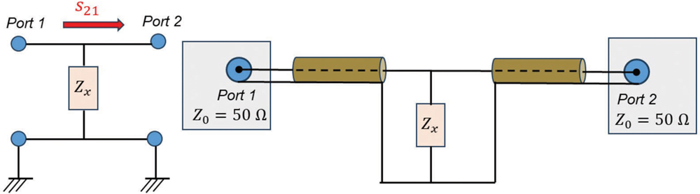
his is the second of two articles devoted to the topic of capacitance impedance evaluation from the S parameter measurements using a network analyzer. The previous article [1] described the impedance measurements and calculations from the S11 parameters using the one-port shunt, two-port shunt, and two-port series methods. This article is devoted to the impedance measurements and calculations from the S21 parameters using the two-port shunt and two-port series methods.

Two-Port Shunt Method
The two-port configuration for a two-terminal DUT is shown in Figure 1.
Two-port shunt configuration
Figure 1: Two-port shunt configuration
Figure 2 shows the transmission line circuit model of this configuration.
Transmission line circuit model of two-port shunt configuration
Figure 2: Transmission line circuit model of two-port shunt configuration
The network analyzer sends the incident waves, vi, (at different frequencies) from Port 1 to Port 2. Between the ports, there is a shunt discontinuity, Zx. Upon the arrival at the discontinuity, the incident waves get reflected and transmitted.

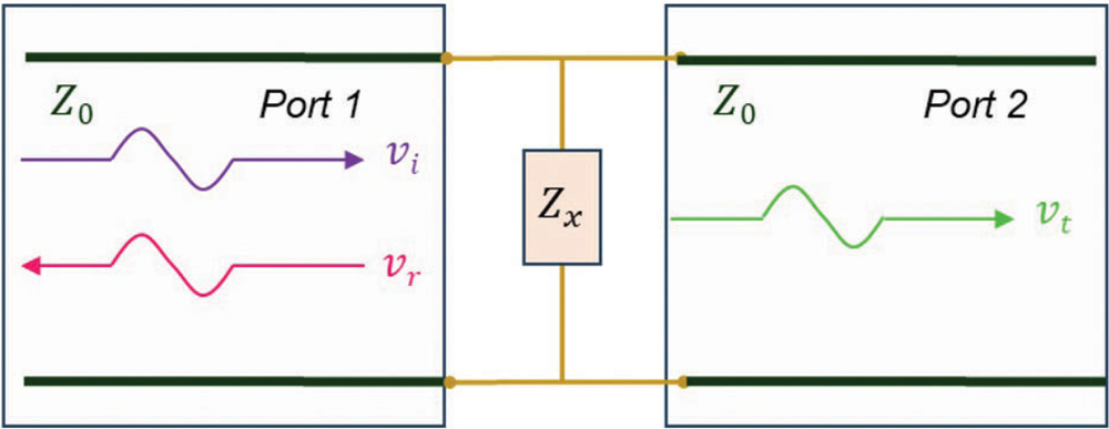
The reflection coefficient at the discontinuity was derived in [1, Eq. (13)] as

equation
The transmission coefficient at the discontinuity, which is equal to s21, is related to the reflection coefficient by
equation
Thus
equation
or
equation
leading to, [2],
equation
Diving into the world of network analyzers, this column uncovers clever techniques for measuring ceramic capacitor impedance—revealing how engineers can precisely decode these tiny electronic components.
Eq. (5) is now solved for Zx in terms of S21.
equation
or
equation
equation
equation
resulting in
equation
Two-Port Series Method
The two-port series configuration for a two-terminal DUT is shown in Figure 3.
Two-port series configuration
Figure 3: Two-port series configuration
For this two-port series configuration, we will use the circuit theory (not the transmission line theory) and the two circuit models shown in Figure 4.
Transmission line circuit models of two-port series configuration: a) Zx = 0, b) Zx ≠ 0
Figure 4: Transmission line circuit models of two-port series configuration: a) Zx = 0, b) Zx ≠ 0
Voltage at port 2, VL1, (with Zx = 0, is obtained from the voltage divider as
equation
Voltage at port 2, VL2, (with Zx ≠ 0, is obtained as
equation
The s21 parameter is determined from
equation
Thus,
equation
or
equation
Eq. (15) is now solved for Zx in terms of S21.
equation
or
equation
equation
equation
resulting in
equation
Impedance Measurement Setup and Results
The impedance measurement setup and the PCB boards are shown in Figure 5. The boards were populated with Murata X7R ceramic capacitors, GCM188R71H472KA37, GCM188R71H473KA55, GCM188R71C474KA55, of the values 4.7 nF, 47 nF, and 470 nF, respectively.
Measurement setup and PCBs
Figure 5: Measurement setup and PCBs
Impedance curves (obtained from the S21 parameter measurements) for a 4.7 nF capacitor are shown in Figure 6.
S21-based impedance curves - two-port series (Eq. 20) vs. two-port shunt (Eq. 10)
Figure 6: S21-based impedance curves – two-port series (Eq. 20) vs. two-port shunt (Eq. 10)
Figure 7 shows the capacitor impedance curve obtained from the Murata Design Support Software “SimSurfing” [4].
C = 4.7 nF, Murata “SimSurfing” impedance curve
Figure 7: C = 4.7 nF, Murata “SimSurfing” impedance curve
The two-port series, two-port shunt, and Murata measurements at 0 dB and self-resonant frequencies for a 4.7 nF capacitor are shown in Table 1.
C = 4.7 nF, Impedances at 0 dB and resonant frequencies
Table 1: C = 4.7 nF, Impedances at 0 dB and resonant frequencies
It is apparent that the two-port shunt measurements, at 0 dB and self-resonant frequencies, are significantly closer to the Murata results, than the two-port series measurements.

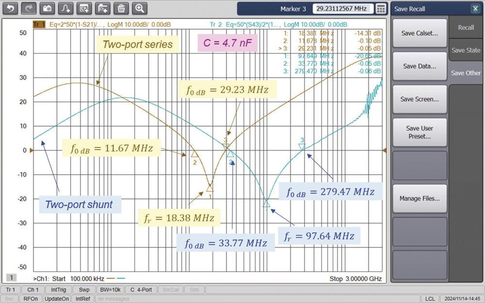
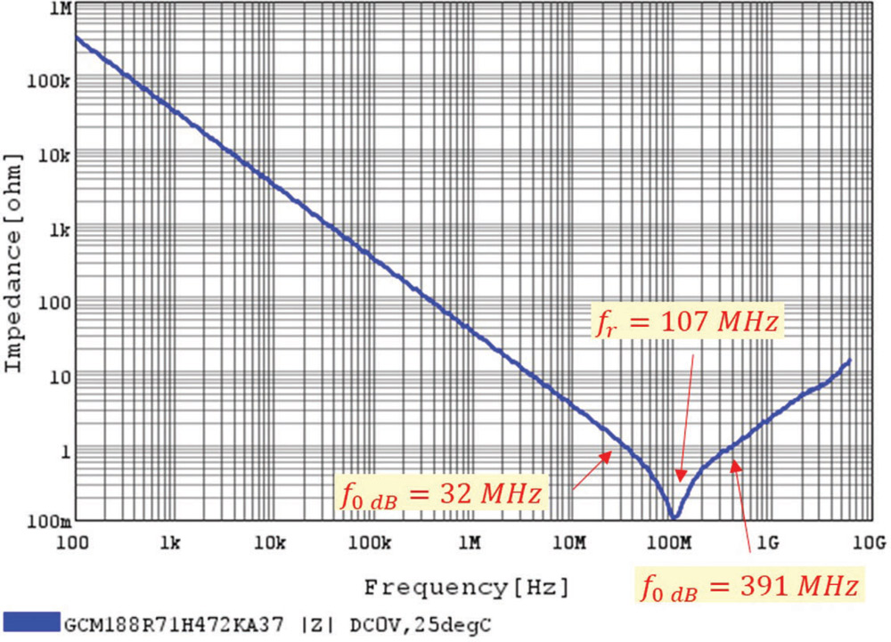
Impedance curves for a 47 nF capacitor are shown in Figure 8.

S21-based impedance curves - two-port series (Eq. 20) vs. two-port shunt (Eq. 10)
Figure 8: S21-based impedance curves – two-port series (Eq. 20) vs. two-port shunt (Eq. 10)
Figure 9 shows the Murata impedance curve.
C = 47 nF, Murata “SimSurfing” impedance curve
Figure 9: C = 47 nF, Murata “SimSurfing” impedance curve
The two-port series, two-port shunt, and Murata measurements at 0 dB and self-resonant frequencies for a 47 nF capacitor are shown in Table 2.
C = 47 nF, Impedances at 0 dB and resonant frequencies
Table 2: C = 47 nF, Impedances at 0 dB and resonant frequencies
Again, the two-port shunt measurements, at 0 dB and self-resonant frequencies, are significantly closer to the Murata results than the two-port series measurements.

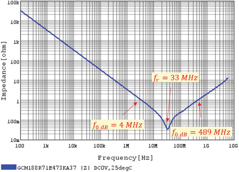
Impedance curves for a 470 nF capacitor are shown in Figure 10.

S21-based impedance curves - two-port series (Eq. 20) vs. two-port shunt (Eq. 10)
Figure 10: S21-based impedance curves – two-port series (Eq. 20) vs. two-port shunt (Eq. 10)
Figure 11 shows the Murata impedance curve.
C = 470 nF, Murata “SimSurfing” impedance curve
Figure 11: C = 470 nF, Murata “SimSurfing” impedance curve
The two-port series, two-port shunt, and Murata measurements at 0 dB and self-resonant frequencies for a 470 nF capacitor, are shown in Table 3.
C = 470 nF, Impedances at 0 dB and resonant frequencies
Table 3: C = 470 nF, Impedances at 0 dB and resonant frequencies
Once again, the two-port shunt measurements, at 0 dB and self-resonant frequencies, are significantly closer to the Murata results, than the two-port series measurements.

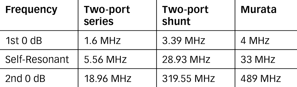
The overall conclusion is that the two-port shunt method is the most accurate method for the capacitor impedance evaluation from S21 parameter measurements.

References
  1. Bogdan Adamczyk, Patrick Cribbins, and Khalil Chame, “Capacitor Impedance Evaluation from S Parameter Measurements – Part 1: S11 One-Port Shunt, Two-Port Shunt, and Two-Port Series Methods,” In Compliance Magazine, February 2025.
  2. Keysight Application Note, Impedance Measurements of EMC Components with DC Bias Current.
  3. Microwaves & RF Application Note, Make Accurate Impedance Measurements Using a VNA.
  4. Murata Design Support Software “SimSurfing.”
Share this story:
Bogdan Adamczyk headshot
Dr. Bogdan Adamczyk is professor and director of the EMC Center at Grand Valley State University (http://www.gvsu.edu/emccenter) where he performs EMC educational research and regularly teaches EM/EMC courses and EMC certificate courses for industry. He is an iNARTE-certified EMC Master Design Engineer. He is the author of two textbooks, “Foundations of Electromagnetic Compatibility with Practical Applications” (Wiley, 2017) and “Principles of Electromagnetic Compatibility: Laboratory Exercises and Lectures” (Wiley, 2024). He has been writing “EMC Concepts Explained” since January 2017. He can be reached at adamczyb@gvsu.edu.
Patrick Cribbins headshot
Patrick Cribbins is pursuing his Bachelor of Science in Electrical Engineering at Grand Valley State University. He currently works full time as an Electromagnetic Compatibility Engineering co-op student at E3 Compliance, which specializes in EMC and high-speed design, pre-compliance testing and diagnostics. He can be reached at patrick.cribbins@e3compliance.com.
Khalil Chame headshot
Khalil Chame is pursuing his Bachelor of Science in Electrical Engineering at Grand Valley State University. He currently works full time as an Electromagnetic Compatibility Engineer co-op student at E3 Compliance, which specializes in EMC and high-speed design, pre-compliance and diagnostics. He can be reached at khalil.chame@e3compliance.com.