Correlation Between Insertion Loss and Input Impedance of EMC Filters

EMC concepts explained

Part 2: π and T Filters

his is the second of a three-article series devoted to the correlation between the insertion loss and input impedance of passive EMC filters. In the first article, [1], LC and CL filters were discussed. This article focuses on π and T filters. Analysis, simulation, and measurement results show that the frequencies at which the insertion losses of these filters are equal are the same frequencies at which the input impedances are equal. These frequencies define the regions where one filter configuration outperforms the other (with respect to the insertion loss). To determine these regions analytically, we compare the input impedances of the two filters. The next article will focus on cascaded LC and CL configurations.

INPUT IMPEDANCE TO THE π FILTER

The input impedance,

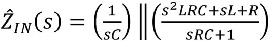
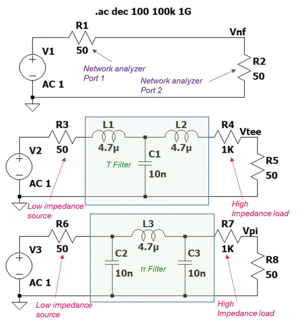
_IN , to the π filter is calculated from the circuit shown in Figure 1.

The equivalent impedance of the parallel RC configuration is

(1)

This impedance is in series with the impedance of the inductor

(2)

which, in turn, is parallel with the impedance of the capacitor. Thus, the input impedance to the filter is

(3)

or [2],

(4)

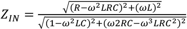
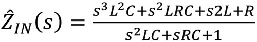
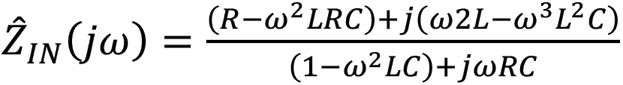
or, in terms of the frequency

(5)

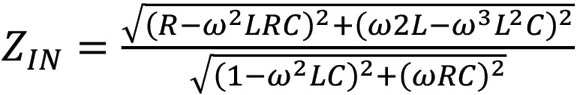
The magnitude of the input impedance is

(6)

Figure 1: Input impedance to the π filter

Input Impedance to the T Filter

The input impedance,

_IN , to the T filter is calculated from the circuit shown in Figure 2.

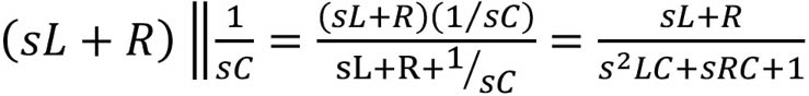
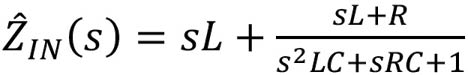
The equivalent impedance of resistor/inductor in parallel with the capacitor is

(7)

Thus, the input impedance to the filter is

(8)

or, [2],

(9)

or, in terms of the frequency

(10)

The magnitude of the input impedance is

(11)

π FILTER VS. T FILTER – INPUT IMPEDANCE – SIMULATIONS AND CALCULATIONS

Let’s look at the input impedances of the two filters. The simulation circuit for this comparison is shown in Figure 3.

The input impedances of the two filter configurations are shown in Figure 4.

Figure 2: Input impedance to the T filter

Figure 3: Simulation circuit for comparison of input impedances

Figure 4: Simulation results: Input impedance – π filter vs T filter

Note that the two input impedances are equal at two frequencies: 733.81 kHz and 1.276 MHz.

Next, let’s calculate the frequency at which the input impedances of the two filters are equal. Equating the expressions in equations (6) and (11) produces

(12)

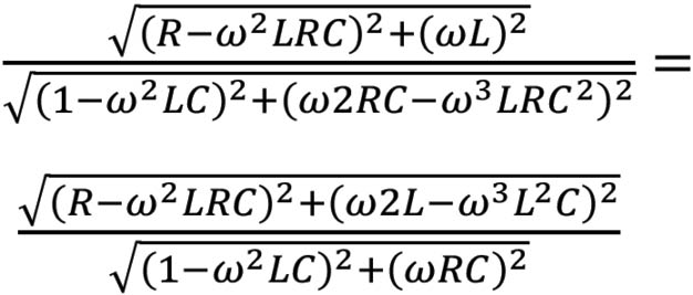
This equation can be solved for ω, [2], resulting in

(13a)

(13b)

The corresponding frequencies in Hertz are

(14a)

(14b)

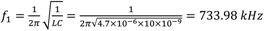
which are consistent with the values obtained from the simulation in Figure 4.

π FILTER VS. T FILTER – INSERTION LOSS – SIMULATIONS AND MEASUREMENTS

Figure 5 shows the simulation circuit used for the comparison of insertion losses, [3].

The simulation results are shown in Figure 6.

At 734 kHz and 1.27 MHz, the insertion losses of the two filters are equal. These are the same frequencies at which the input impedances of the two filters were equal!

Figure 5: Simulation circuit for comparison of insertion losses

Figure 6: Simulation results: Insertion loss – π filter vs. T filter

Note that up to the frequency of 734 kHz, the insertion loss of an π filter is larger than that of the T filter. Between the frequencies of 734 kHz and 1.27 MHz, the insertion loss of the T filter is larger. Beyond the frequency of 1.27 MHz, the insertion loss of the π filter is again larger.

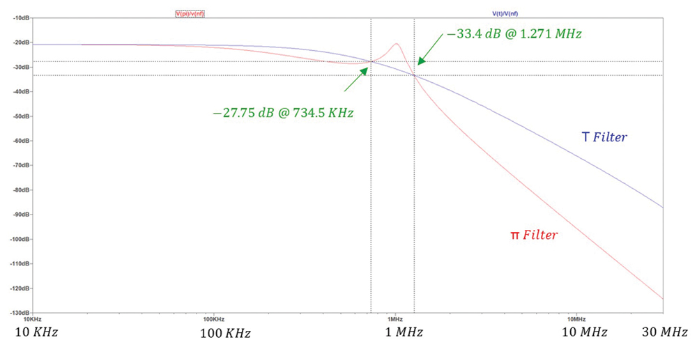
Again, [1], we have arrived at a very important observation: once the filter components values L and C are chosen, we can determine the frequencies at which the insertion losses of π and T filters are equal. These are the frequencies at which the input impedances are equal, given by Equations 14a and 14b.

Figure 7: Measurement setup: Insertion loss – π filter vs. T filter

Figure 8: Measurement results: Insertion loss – π filter vs. T filter

To verify the simulation results of the insertion loss, the measurement setup shown in Figure 7 was used. The measurement results are shown in Figure 8.

Note that the measurement results agree with the calculated and simulated results.

References

Bogdan Adamczyk and Jake Timmerman, “Correlation between Insertion Loss and Input Impedance of EMC Filters – Part 1: LC and CL Filters,” In Compliance Magazine, October 2023.
Bogdan Adamczyk, Principles of Electromagnetic Compatibility: Laboratory Exercises with Lectures, Wiley, 2024.
Bogdan Adamczyk and Brian Gilbert, “EMC Filters Comparison Part II: π and T Filters,” In Compliance Magazine, January 2020.

Share this story:

Dr. Bogdan Adamczyk is professor and director of the EMC Center at Grand Valley State University (http://www.gvsu.edu/emccenter) where he regularly teaches EMC certificate courses for industry. He is an iNARTE certified EMC Master Design Engineer. Prof. Adamczyk is the author of the textbook “Foundations of Electromagnetic Compatibility with Practical Applications” (Wiley, 2017) and the upcoming textbook “Principles of Electromagnetic Compatibility with Laboratory Exercises” (Wiley 2023). He can be reached at adamczyb@gvsu.edu.

Jake Timmerman is an EMC Engineer at E3 Compliance, which specializes in EMC & SIPI design, simulation, pre-compliance testing, and diagnostics. He received his B.S.E in Electrical Engineering from Grand Valley State University. Jake participates in the industrial collaboration with GVSU at the EMC Center. He can be reached at jacob.timmerman@e3compliance.com.

Back to Issue