urrent probes are used to perform conducted emission (CE) measurements in accordance with various product standards like CISPR 11, CISPR 25, or CISPR 32. All these product standards refer to the basic standard CISPR 16-1-2 (2014), which includes normative specifications for current probes in clause 5.1.3. Some of the current specifications include:
- Insertion impedance: 1 Ω impedance maximum;
- Transfer impedance: 0.1 Ω to 5 Ω in the flat linear range; 0.001 Ω to 0.1 Ω below the flat linear range (current probe terminated into 50 Ω load);
- Added shunt capacitance: less than 25 pF between the current probe housing and measured conductor; and
- Frequency response: Transfer impedance is measured over a specified frequency range to calibrate the probe; the range of individual probes is typically 10 kHz to 100 MHz, 100 MHz to 300 MHz, and 200 MHz to 1,000 MHz.
Furthermore, work related to the definition and measurement methods for the specification “insertion impedance” was initiated by CISPR/A/WG1 in 2017 to address the current lack of a standardized measurement method.
This article will discuss the following aspects related to the above CISPR 16-1-2 requirements, including:
- The appropriateness of the 1 Ω Insertion Impedance specification in the context of its impact on both the calibration process and for measurements using a simple CE test configuration, per CISPR 25 (see Reference 1);
- Meaning and usefulness of the shunt capacitance specification; and
- Practical purpose and usefulness of various inferred “limits” for current probe transfer impedance versus frequency, as documented in Reference 5.
The situation is compounded by the fact that for some specifications no definition for “insertion impedance” exists, and no agreed-on measurement methods are made available to determine the values of specifications like insertion impedance or “shunt capacitance.”
Additionally, there is a misalignment between CISPR 16‑2-1 and product standards regarding the frequency range for specifications. Most product standards use the current probe in the frequency range of 150 kHz to 30 MHz for conducted emission measurements, with the exception of CISPR 25, which calls out a maximum frequency of 245 MHz for current probe measurements. CISPR 16-1-2, on the other hand, defines several frequency ranges for the specification of frequency response, up to 1 GHz.
This situation has created considerable confusion among users as to how rigorously to apply the current probe requirements in CISPR 16-1-2 when purchasing current probes or calibration services for current probes. Some concerns were formally raised by some CISPR product committees like CISPR/D and CISPR/A that started the process to formally address these concerns. Several aspects are currently under discussion and the three topics previously outlined do serve as input to the resolution of currently existing problems related to current probe specifications.
In CISPR/A, three different methods to measure the insertion impedance of current probes were proposed in 2018. However, these methods only cover the frequency range of up to 30 MHz, which excludes a large portion of the frequency range stipulated by CISPR 25 (up to 245 MHz). The rationale for the limitation of the frequency range to 30 MHz was given as the requirement for the calibration fixture dimensions needing to be small compared to the wavelength. This explanation is not obvious since the wavelength at 30 MHz is 10 m, and all calibration fixtures have dimensions that are more than an order of magnitude smaller for the current probes used for conducted emission measurements in accordance with CISPR product standards.
The three proposed measurement methods introduced by CISPR/A Working Group 1 are addressed in the following sections.
One-Port Reflection Method
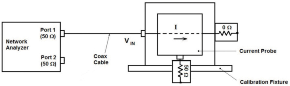
While the suggested principle is plausible, it is unclear why the output of the fixture is terminated in a short and not in 50 Ω. In case of a short, the network analyzer measures a very high reflection in case of an empty fixture and with the probe placed inside the fixture. It seems preferable to measure close to the system impedance of 50 Ω since the uncertainty contribution of the network analyzer is minimized in this scenario, which improves the uncertainty of the insertion impedance measurement.
Series-Thru Method
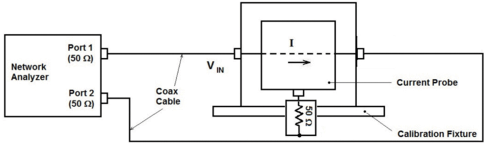
This method seems to be more beneficial compared to the one-port reflection method since the system impedance of 50 Ω is maintained throughout the measurement process.
Shunt-Thru Method
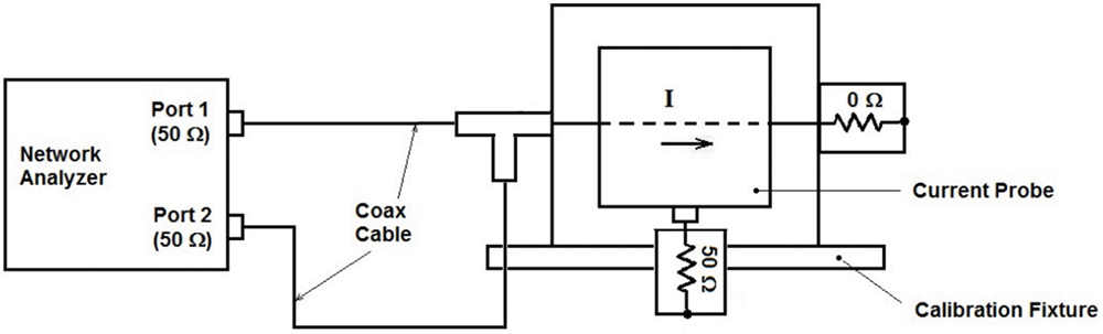
In the description previously provided, it was unclear where the full two-port calibration of the network analyzer is performed. Is the reference plane for the measurement established at the end of the cables without considering the T-connector, or is the T-connector somehow included in the network analyzer calibration process? It seems that this method yields a larger measurement uncertainty since the T-connector can cause coupling of the source signal (Port 1) directly to the measurement channel (Port 2), and the reflected signal from the short termination can reflect back into the source channel. As stated in the document, the influence of the calibration fixture on measurement results was unknown, which seems problematic since no details of the fixture were provided in the contribution.
Further work in CISPR/A Working Group 1, completed in 2021, expands on the initial work regarding measurement methods for insertion impedance. The originally proposed measurement methods were repeated, using a calibration fixture suggested by the current probe manufacturer for the probe under investigation. Based on the calculated measurement uncertainty associated with each method, the “shunt-thru method,” using a transmission measurement, was identified as the most accurate method to determine insertion impedance. It is to be noted that the measurement uncertainty was only based on the contribution of the network analyzer, not considering possible fixture influences. It would be beneficial to investigate the influences by using different fixtures to be able to determine the impact on the insertion impedance measurements.
While the “shunt-thru method” to 30 MHz looks like the most promising method from a consistency and uncertainty standpoint, the results, presented up to 100 MHz, indicate two things of interest:
- First, the measured insertion impedance is about 3 Ω and rises with increasing frequency, which does not comply with the current specification; and
- Second, the measured insertion impedance appears to begin diverging between S11,22 and S21,12 at 30 MHz. This appears to illustrate the difficulty that will be encountered at frequencies above 100 MHz and most certainly at 1 GHz. The divergence shown in the resultant plot infers a fundamental problem in defining the “proper” method, particularly in light of the maximum test frequency range used by CISPR 25.
- A variety of calibration fixtures were used by participants of the RRT. Only one participant used the calibration fixture suggested by the manufacturer of the current probe.
- On the one hand, this would seem to violate a round-robin concept of all participants using the same hardware (not considering the probe electronics) to isolate differences in how various laboratories execute a given test method. On the other hand, it points out the importance of using a proper test fixture (recommended by the probe manufacturer).
The RRT summary report acknowledges the fixture issue as the “dominating influence above 600 kHz” and reinforces the notion that the use of the proper calibration fixture is crucial. Furthermore, one conclusion drawn in this paper states that “the measurement method is effective to measure Insertion Impedance of current probes.” It is unclear how this general conclusion can be drawn since the measurements were made only up to 100 MHz, not covering the full frequency range to 245 MHz in CISPR 25. In addition, as stated before, the fixture has a significant impact. Therefore, the suitability of the method is dependent on the use of a “proper” fixture.
Since the insertion impedance discussion tends to be more focused on the calibration aspect, our technical experts elected to focus initially on the calibration perspective, which is discussed later in this article.
Figure 4 shows the basic test setup we used for our insertion impedance investigations, which includes the following steps:
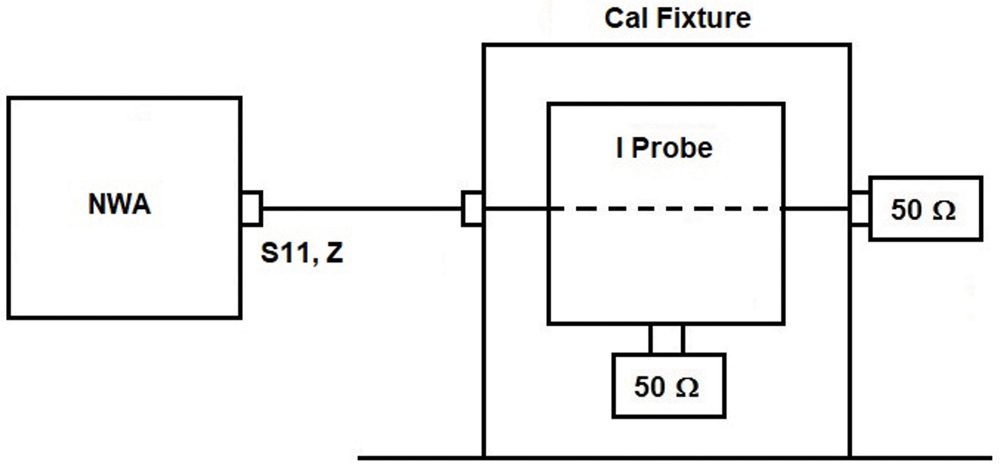
- An S11 calibration was performed with short, open load at the end of the measurement cable with the network analyzer configured to measure impedance Z based on S11;
- The current probe was removed from the calibration fixture;
- A network analyzer sweep was performed and saved;
- The current probe was installed in the calibration, and another network analyzer sweep was performed and saved; and
- The difference between the two network analyzer sweeps was calculated as the measured insertion impedance.
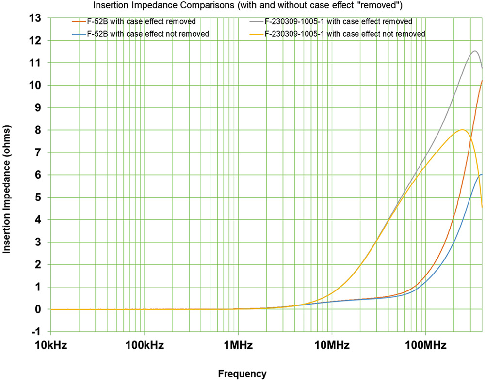
References 3 and 4 seem to be typical attempts to model current probes. The primary focus is on the equivalent electrical circuit comprised of the electronics of a current probe. The probe case is not included in the modeling. The previously described measurement treated the probe electronics and its case as an integrated item. With the probe case being a major point of interest, we performed a variety of insertion impedance measurements with and without the use of an empty probe case in an attempt to remove the case influence on the measured insertion impedance.
Both types of insertion impedance measurements were made on two different probes. The first is a widely used current probe that has a nominal transfer impedance of about +13 dB ohms from about 5 MHz to 400 MHz. The second probe was one that has a nominal transfer impedance > =20 dBΩ from about 50 MHz to 1000 MHz.
- Inherent transfer impedance;
- Size of probe case; and
- Maximum frequency of interest.
From Figure 13 in CISPR 25 (2021), it is apparent that a loop is formed by the equipment under test (EUT), the load simulator, the interconnecting wire, and the ground plane. It is not clear if the two artificial networks and the DC power supply are part of this loop or if the load simulator provides some electrical isolation between the EUT and power and artificial networks.
Reference 5 investigates the “influence of termination impedance on conducted emissions in automotive high voltage networks.” In this document, the authors started with an equivalent circuit that consisted of a loop formed by the DC power (+) side, through a line impedance stabilization network (LISN), through the EUT, and then back to the DC power (-) side after passing through a second LISN.
Both of these examples point to the use of an electrical loop as a starting point to look at loop impedance versus frequency and how the potential addition to this loop impedance through the presence of a current probe might be important.
An investigation was started by combining the two concepts into the configuration shown in Figure 6.
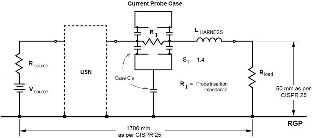
- A DC power source assumed to have some inherent source impedance/resistance
- An optional LISN on the (+) side
- A cable harness over a reference ground plane, as per CISPR 25, specified as follows:
- The length of harness set at 1700 mm as per CISPR 25;
- The height of harness above ground plane set at 50 mm as per CISPR 25;
- The harness outer diameter is a variable depending on DC current flowing through harness;
- The harness suspended above ground plane with a dielectric material having a relative permittivity <= 1.4, as per CISPR 25; and
- Harness introduces a series inductance to the loop impedance.
- A load impedance is assumed to be set by the operating current in the harness and DC power source voltage
- Shunt capacitance
- CISPR 16-1-2 states that the probe case to wire under test is to be considered. However, it is unclear if the assumption is that this capacitance somehow compromises the measuring ability of the probe (i.e., affecting its transfer impedance) or if this requirement infers that this capacitance is then coupled to reference ground. Figure 6 shows both types of capacitances.
The highest operating voltage for an electrical vehicle that we are aware of is 800 V1. Current probe users have expressed interest in current probes with a DC current handling of up to 1000 A. For simplicity reasons, it is assumed that 800 VDC delivers 800 A, which infers a DC loop impedance of 1 ohm. In Figure 6, this 1 Ω would be the sum of Rsource and Rload.
To establish a nominal value for LHARNESS in Figure 6, the wire gage rated for 800 A was researched and found to be 750 AWG2, which has a diameter of about 30 mm. Using “All About Circuits”3, we established a harness inductance for this diameter wire, 1700 mm long and 50 mm above a ground plane over a dielectric material, and having a relative permeability of 1.4, yielding a value for LHARNESS of about 0.89uH.
It is obvious that LHARNESS will start to dominate the loop impedance at some point, depending on frequency. If it is assumed that the LHARNESS impedance is to be at least 10 times the presumed 1 Ω insertion impedance, introduced by the current probe, for the insertion impedance to be negligible, this leads to:
2 * π * f * LHARNESS, = 10 Ω, therefore f = 1.43 MHz
Based on the consideration above, the following can be concluded:
- For a very low loop impedance, the harness inductance will start to dominate the total loop impedance above approximately 1.43MHz;
- As the operational current drops, the load resistance Rload will increase, which further mitigates any impact of the current probe insertion impedance; and
- If one 50 Ω/5 uH LISN, as defined in CISPR 16‑1‑2, is included in the series loop impedance, the loop impedance will only increase; at 150 kHz, this LISN would add an impedance of about 4.7 Ω. At the frequency 1.43 MHz previously calculated, the LISN added impedance is about 33 Ω. If a second LISN is included in the series impedance, the impedance will increase further, reducing any impact of the insertion impedance.
Summarizing these factors, it is not clear why the specified insertion impedance of 1 Ω for current probes will ever have any serious impact on any CE test per CISPR 25 at test frequencies above a few 10s of MHz (and possibly much lower) and especially considering the upper usage frequency of 1 GHz, as inferred by CISPR 16-1-2.
Addressing the effect of the capacitance shown in Figure 6:
-
CISPR 16-1-2 defines this shunt capacitance between the probe case to the wire under test. The origin of and rationale for this requirement is not known. If the assumption is that this capacitance is compromising the transfer impedance of the current probe, then it seems that this effect would be accounted for during routine probe calibration. If the intent is that this capacitance is possibly affecting the CE measurements, then this capacitance would be a presumed shunt to ground for measured CE signals.
At 1 GHz, 25 pF is about 6.4 Ω. Based on a parallel argument to that made previously regarding the impact of LHARNESS, it is not clear why the impact of this capacitance wouldn’t also be minimized. For example, using the 1.43 MHz frequency, estimated in the above example, this capacitive impedance is about 4500 Ω; it doesn’t seem a likely problem in a real test setup.
- No method for measuring this capacitance has been defined. De facto, the inference is that the shunt capacitance would have to be measured in the test setup itself, to “verify” compliance of the current probe. It does not seem practical to define such an in-situ specification (which indicates a pass/fail for the current probe and/or the test configuration), especially at high frequencies where suitable measurement devices either don’t exist or are expensive to implement
- Therefore, it is not evident that such a specification is really needed.
The document prepared by CISPR/D in 2023 further reinforces this notion by showing a variety of current probes, separated into frequency ranges where the probe meets stated specifications, along with some limits for usability. Appendix B.3 of CISPR 16-1-2 infers that the upper “limit” of +15 dBΩ, shown in the CISPR/D document, derives from the notion that a higher transfer impedance automatically exceeds the 1 Ω insertion impedance requirement. This would appear to derive indirectly from the simplified circuit models for a current probe given in Appendix B.2. However, Reference 4, which discusses the wide-band characterization of current probes, states that models based on simple transformer theory may not work above 100 MHz. This reference presents a complicated mathematical method (possibly impractical for the average user to employ) for recovering current probe behavior at higher frequencies up to 3 GHz. Reference 4 also presents some modeling but only up to 100 MHz.
Therefore, it seems unnecessary to establish transfer impedance “limits,” a fact that also causes confusion for users. Furthermore, the frequency response specification infers that the stated frequency ranges are the ones over which current probes should be calibrated, which is simply incorrect and misleading. The current specifications regarding transfer impedance should be removed from the normative part of the standard.
We further suggest revising Appendix B of the standard to provide information about the proper selection of current probes to achieve the necessary test system sensitivity, taking into consideration the current level to be measured, including measuring instrument noise floor, saturation, required resolution bandwidth, etc.
Conclusions
The purpose of the 1 Ω insertion impedance requirement is not obvious. Other test considerations would seem to dominate over any possible impact of a 1 Ω impedance. Furthermore, suggested insertion impedance measurement approaches, presented up to 100 MHz, do not seem to yield results that allow an extension in frequency to ranges required, for example, by CISPR 25 (to 245 MHz). Therefore, it is suggested to remove this requirement from the normative part of CISPR 16-1-2.
Furthermore, the shunt capacitance requirement of 25pF is confusing since it is not clear if this requirement applies to the calibration aspect of current probes or to the use in an actual application. It seems very impractical to have users verify this value in an actual measurement setup. If this requirement is to be interpreted as an aspect of a current probe calibration process, its usefulness is questionable since the calibration setup (using a calibration fixture) will certainly differ from the actual measurement setup that uses a harness, for example. Therefore, it is suggested to remove this requirement from the normative part of CISPR 16-1-2.
It does not seem appropriate for CISPR/A to define frequency ranges for the frequency response of the transfer impedances since there is no basis provided for setting such requirements. These requirements set bounds on a user regarding the selection of a current probe for a specific application. Since there is no basis given for this requirement, it should be removed from the normative part of the standard.
Resolving the issues identified in this article will hopefully allow current probe users to perform measurements in accordance with product standards like CISPR 25 with the sensitivity required.
- CISPR 25 (2021-12)
- CISPR 16-1-2 (2017-11)
- C. F. M. Carobbi and L. M. Millanta, “Circuit Loading in Radio-Frequency Current Measurements: The Insertion Impedance of the Transformer Probes,” IEEE Transactions on Instrumentation and Measurement, vol. 59, no. 1, pp. 200-204, January 2010
- G. Cerri, R. De Leo, V. M. Primiani, S. Pennesi, and P. Russo, “Wide-band characterization of current probes,” IEEE Transactions on Electromagnetic Compatibility, vol. 45, no. 4, pp. 616-625, November 2003
- M. Reuter, S. Tenbohlen, W. Koehler, “Influence of Termination Impedance on Conducted Emissions in Automotive High Voltage Networks,” International Symposium on Electromagnetic Compatibility – EMC EUROPE, September 2012.
Werner Schaefer has 40 years of experience RF/uwave and EMC testing and was involved in the development, marketing, and support of EMC test equipment. He owns Schaefer Associates, a company that provides assessment, training, and consultancy services to the fields of EMC, RF/uwave, and Quality Assurance. Schaefer can be reached at wernerschaefer@comcast.net.