Seventy Years of Electromagnetic Interference Control in Planes, Trains, and Automobiles (and Ships and Spaceships, as well)

Feature Article

Seventy Years of Electromagnetic Interference Control
in Planes, Trains, and Automobiles (and Ships and Spaceships, as well)

Understanding Today’s EMI Limits and Test Methods Begins With Knowing How We Got Here

By Ken Javor

Explanatory Note¹

This is the first in a multi-part series of articles exploring the background of modern electromagnetic interference (EMI) requirements and test methods. In this first part, we’ll cover general topics. Part 2 will address the line impedance stabilization network (LISN) and test methods based on it. Subsequent parts will be devoted to radiated emission control and will address the important topic of “(Re)Discovering the Lost Science of Near Field Measurements.”

In each of these articles, there is a preponderance of references to various military electromagnetic interference specifications.² This should not be interpreted as limiting the subject matter discussed to the military sector. Both aerospace and automotive EMI specifications/standards bear a strong resemblance to military EMI standards, and that resemblance has been tracked over decades as these specifications/standards evolved. That is, commercial aerospace specifications from the 1960s and 1970s look like contemporaneous military specifications, and when the automotive industry later instituted EMI qualifications, those qualifications were similar to contemporaneous military practices.

This is not to say that these industry sectors simply copied military practices. At any particular point in time, radios,³ culprit noise sources, and their installations tend to be similar, causing similar EMI issues and consequently similar EMI controls (limits and test procedures).

1950s EMI test set-up. (Photo courtesy of Ed Price.)

21^st century EMI test chamber. (Photo courtesy of Rohde & Schwarz.)

It is commonplace to contrast military vs. commercial EMI test practices, but that is not a fundamental distinction. Commercial aerospace and automotive EMI test practices have much more in common with military practices than they do with the qualification of consumer items on open area test sites (OATS) or in fully or semi-anechoic chambers (FAC/SAC). The fundamental difference is in installation in a vehicle (usually metal) vs. equipment slated for use in homes, offices, and industrial plants. EMI testing of equipment installed in vehicles requires acknowledgment of the immediate proximity of electrical ground (vehicle structure) and the possibility that vehicle antennas will be placed in close proximity to culprit electrical noise generators.

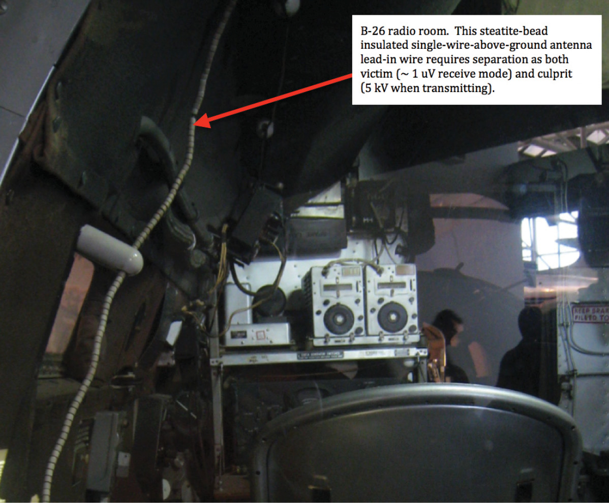
Vehicles of all kinds – even large ships – must countenance culprit-victim separations in the very near field. Not all antenna-culprit separations will be precisely one meter, and while one-meter measurements are not scalable as are far-field measurements, the vehicle EMC verification process takes that into account.

The subject matter in this multi-part series of articles has been limited to a length and level of detail appropriate for magazine publication. An expanded discussion of these topics will be posted on the author’s website in the near future.⁴ Sections with significantly expanded coverage in the website version are flagged with an asterisk (*).

Introduction

This year marks the seventieth anniversary of several developments that culminated in the birth of the modern EMC discipline. EMI specifications released in late 1952 and throughout 1953 incorporated technical improvements in test equipment and measurement procedures that previously didn’t exist, or existed in a more primitive state.

Prior to the end of World War II, there were no EMI specifications at all.⁸ Instead, there were specifications describing how to verify that integrated vehicles had sufficient EMI suppression to ensure the vehicle’s suite of radios would operate free from interference.

We shall take as an example MIL‑I‑6181B, whose seventieth anniversary is this month.⁵ While the improvements in MIL‑I‑6181B showed up in multiple contemporaneous specifications, MIL‑I‑6181B has two very important aspects that the other specifications don’t. The MIL-I-6181 series (1950 – 1967) ran right up until MIL‑STD‑461 superseded all Service-specific EMI specifications, whereas most of the other specifications dead-ended prior to that. MIL‑I‑6181B changes stood the test of time.

Secondly, we have a rationale or white paper report detailing the engineering behind the radiated emissions portions of MIL‑I‑6181B. NADC-EL-5515 precisely documents the problem and the solutions developed, and the process between problem and solution.⁶ This report, authored in 1955 by William Jarva of the Naval Air Development Center, serves as a Rosetta Stone, unlocking the mystery behind the limits and test methods used to control unintentional radiated emissions. It should be required reading for anyone involved in vehicle EMC.

The Way Things Were (pre-1967)

Some brief background is in order for those readers unfamiliar with anything before the Tri-Service MIL‑STD‑461 (1967 forward).⁷

Prior to the end of World War II, there were no EMI specifications at all.⁸ Instead, there were specifications describing how to verify that integrated vehicles (planes, trains, automobiles, ships, and submarines) had sufficient EMI suppression to ensure the vehicle’s suite of radios would operate free from interference. Such EMC specifications were accompanied by quite sophisticated handbooks and suppression specifications showing proper installations of both radio and non-radio electrical equipment so as to minimize the probability of radio frequency interference. Eventually, it was determined that designing a certain amount of suppression and immunity into electrical and electronic equipment was more efficient overall than trying to solve everything during vehicle integration, and this gave birth to JAN-I-225, the first EMI specification.⁹

From 1945 to 1967, there were individual Service-unique EMI specifications. During that period, there were multiple standards that were similar to but slightly different from each other. So test engineers had to have intimate familiarity with each of as many as a dozen specifications and their various nuances, and also access to and knowledge of different fully manual EMI receivers required in various specifications. Any reader who works for a living in the business of EMI testing should be grateful for a single Tri-Service specification!¹⁰

While MIL‑I‑6181B evolved from a predecessor specification, it was revolutionary in many aspects.^11,12

Technological Changes

Two big technology changes appeared between 1950 and 1953. These were the widespread adoption of the 5 uH LISN, still in use in aerospace and automotive EMI practice to the present day, and the commercial availability of the AN/PRM-1 EMI receiver. Developed by the Stoddart Aircraft Radio Company circa 1950, this was the first EMI receiver operating below 30 MHz (conducted emission and rod antenna frequency range) with a peak detector.

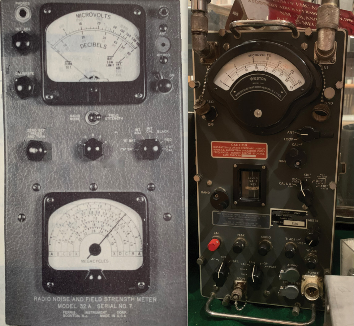
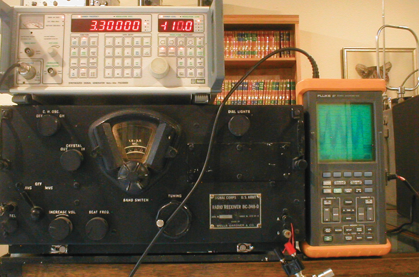
Both of the EMI receivers shown in Figure 1 were designed for direct attachment of a 41” rod. Only the AN/PRM-1 has a (slide-back) peak‑detecting capability.¹³ The Ferris meter was much older, dating from 1932. According to Al Parker, the AN/PRM-1 was developed between the end of WWII and 1950.¹⁴

Figure 1: Ferris 32-A and Stoddart’s AN/PRM-1 EMI receivers. (Photo courtesy of the Museum of EMC Antiquities.)

The advent of an EMI receiver with a peak detector operating in the conducted emission measurement frequency range meant it was no longer necessary to count the repetition rate of broadband impulses in order to apply correction factors based on the rep rate. This resulted in a less complex measurement set-up, and much less time analyzing EMI signatures.

(The 5 uH LISN was such an important development that it gets its own separate discussion in Part 2 of this article series.)

Bandwidth Matters

Discrimination between narrow and broadband interference sources is dealt with in detail in MIL‑I‑6181B, whereas the issue had been largely ignored before that. That is, where multiple EMI receivers are available, utilizing different measurement bandwidths, some with and some without peak detection, the measurement of broadband signals must be normalized on a per-unit bandwidth basis. Not only that, but the BC-348Q radio, which was the actual victim used to determine the limit, had a bandwidth of about 2 kHz, whereas the Ferris meter had a 10 kHz bandwidth.^15,16 Further, if a peak detector is not available, the response of the EMI receiver is dependent on the repetition rate of the impulses, so that a repetition rate correction factor curve is provided in MIL‑I‑6181B.

This was the inception of narrowband-broadband discrimination and separate limits. While that is largely obsolete today, it is not without merit. The demise of separate limits in MIL‑STD‑461D in 1993 was largely based on the perception that not enough people were doing it correctly, and the procedure had to be simplified to the point where people were all doing it the same way.¹⁷ Hence, single‑bandwidth measurements are ubiquitous today. These rely on CISPR 16-1 specifying these bandwidths for all EMI receivers, and also on these bandwidths being representative of those used by the actual radios protected by emission limits.

But the failure of such simplifications is evident in cases where multiple bandwidths are in use by various radio services. For instance, dithered clocks spread clock harmonics across several measurement bandwidths, decreasing the signal measured in any one bandwidth. This is a fine design technique as long as the radio protected from such interference has a bandwidth similar to that mandated by CISPR 16‑1. But when the victim radio has a much larger bandwidth, such as broadcast television, then even the dithered clock energy falls within a single channel. So even though the dithered clock amplitude is under the limit measured with a 120 kHz bandwidth, such signals can cause TVI. If a separate bandwidth such as 1 MHz or better yet 6 MHz were used, that would tell the tale for the TV receiver.

Figure 2: Unshielded antenna lead-in WWII-era B-26 bomber radio room. The BC-348 radio to which it connects is forward of the seat back and below silver-colored radio equipment in the rack. BC-348 is shown to better effect in Figure 4. (Photo taken by the author at Smithsonian National Air & Space Museum.)

Figure 3: The circular ceramic is the fuselage penetration treatment for the unshielded antenna lead-in. It wasn’t just the 5 kV transmit voltage driving the treatment, but also the high frequency requiring control of shunt capacity. Control of shunt capacity was provided within the aircraft by ceramic standoffs. The 2” distance between the base and the hole is the basis for the 2” (5 cm) standoff requirement in all subsequent EMI specifications and standards. (Photo courtesy of the Museum of EMC Antiquities.)

Nowadays this is easily achieved with FFT or time-domain type receivers, which can look at a very large spectrum and then digitally simulate what would be measured using various smaller bandwidths and detectors, all from a single high-speed sweep. It may be time to take a look at this 1953 innovation once again.

The Answer to an Oft‑Posed Query

Sometimes a complex subsystem has a great number of attached cables. MIL‑STD‑462D (and subsequent versions of MIL‑STD‑461 that rolled MIL‑STD‑462D into MIL‑STD‑461) requires that the cable closest to the front edge of the ground plane be 10 cm back from the edge, and then 2 cm between each succeeding cable and the last.¹⁸ With enough attached cables, the ground plane may not provide enough depth. It is often asked if the first cable may be pushed closer to the edge to free up some room. Or is it better to bunch cables closer than 2 cm separation?

Another question less often posed is if the installation is known to hold cables much closer to the structure than 5 cm, can the test set-up simulate that?

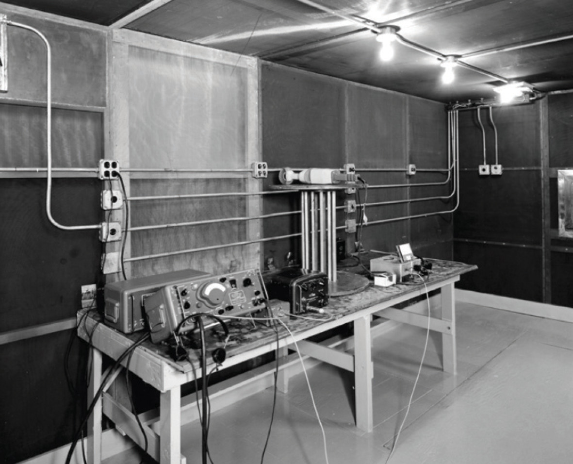
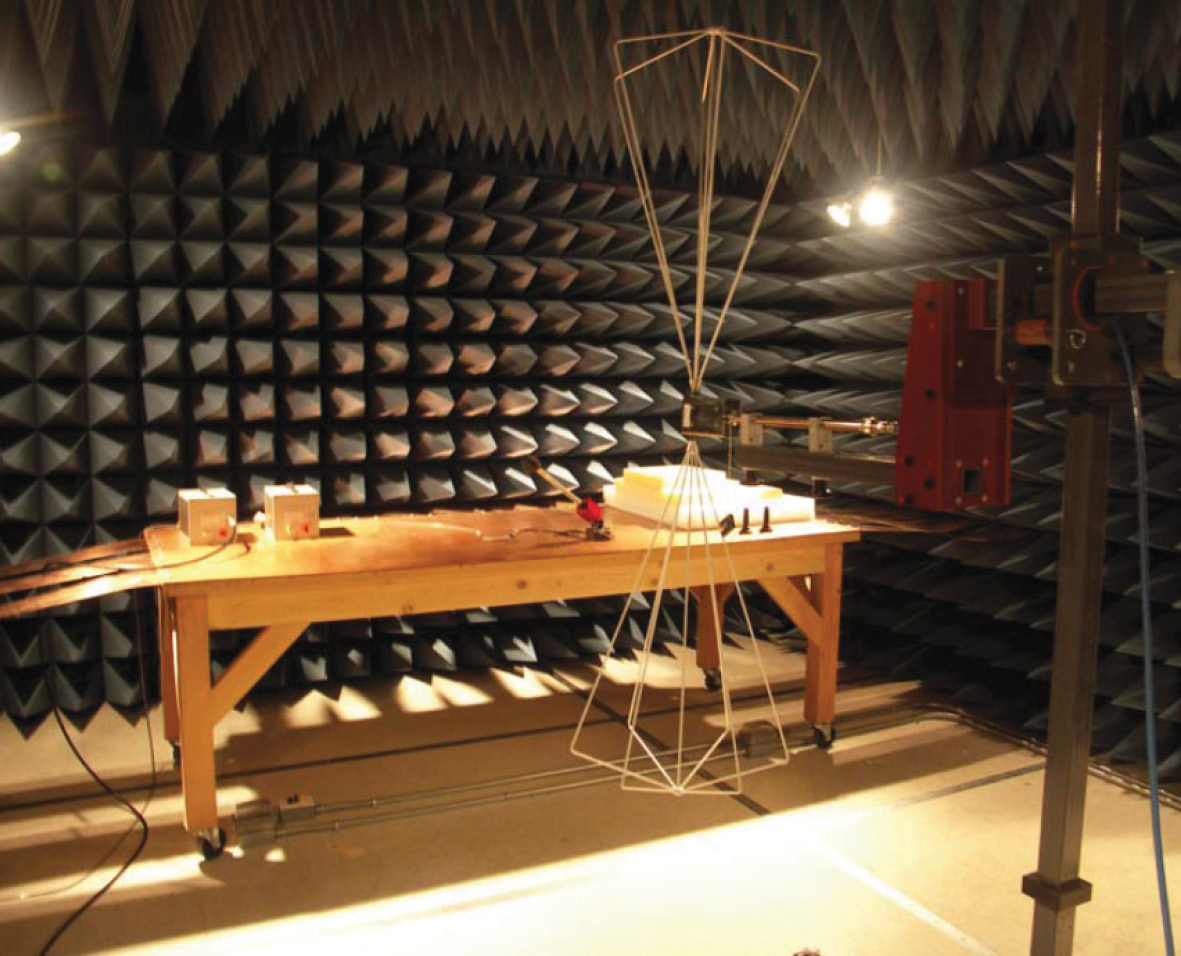
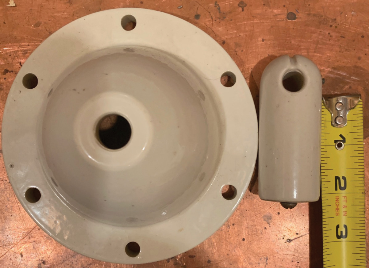
The closer that first cable is to the ground plane edge, the more efficiently it radiates (RE102), and the more efficiently a radiated field can couple to it (RS103) – hence the need for standardization. As illustrated in Figures 2 and 3, the separation of cables on standoffs holding them 2” (now 5 cm) above a ground plane is first found in MIL‑I‑6181B. Previously in JAN-I-225 (and thus MIL-I-6181 which relied on JAN-I-225 for test procedures) it was a quarter-inch over the ground plane. Separation between cables was also 2”, but that has decreased to 2 cm in MIL‑STD‑461. For a “seeing is believing” demonstration of the reason behind the cable-to-cable separation requirement, see https://youtu.be/uiyLQpsOqX8. Armed with this information, the reader may now make informed decisions.

Figure 4: The author’s unaltered BC-348Q radio, the specific radio model whose performance characteristics drove the emissions and susceptibility requirements in MIL‑I‑6181B below 20 MHz. The photo shows a noisy but audible response to a 1 kHz modulated radio frequency signal at a level of – 3 dBuV. (Photo courtesy of the Museum of EMC Antiquities.)

Evolution of Conducted Emission Limits*

As evidenced in the above-cited YouTube video, the BC-348 radio had very little EMI filtering on its 28 Vdc power input and was susceptible to very low levels of RF noise on its power input. MIL‑I‑6181B conducted emission limits protecting the BC-348 radio are portrayed in Figure 5, with the superseding CE03 limits superimposed. MIL‑I‑6181B imposed a value of 1 mV for conducted susceptibility. This level increased to 100 mV in subsequent releases of MIL-I-6181, and then up to 1 volt in MIL‑STD‑461.

These measures were taken to gradually force improvement in power-line EMI filtering. At the same time, the very stringent conducted emission limits found in MIL‑I‑6181B had to be levied to protect the existing inventory of installed radios with little or no power-line filtering. As time went by, these stringent conducted emission limits were relaxed as the inventory of obsolete susceptible receivers declined, being replaced by receivers that met the higher level conducted susceptibility limits.

Figure 5: MIL‑I‑6181B conducted emission limits, with superimposed MIL‑STD-461 CE03 limits.

But the conducted emission limits could not be relaxed as much as the conducted susceptibility limits had strengthened, because conducted emissions cause radiated emissions, and radiated emissions must be controlled to protect antenna-connected receivers. The narrowband CE limit in radio bands were relaxed to about 1 mV, where the -6181B conducted susceptibility started out. This amounted to at most a 26 dB relaxation. Paradoxically, the broadband limit became more stringent. The MIL‑I‑6181B broadband limit protected the 2 kHz BC-348 radio bandwidth. Later broadband limits protected wider bandwidths.

Controlling Radiated Emissions – The Science of Near-Field Measurements*

A huge advance in -6181B is described in detail in NADC-EL-5515. This is the concept that, when making near-field measurements, the way the measurement is made materially affects the result. The type of antenna, its physical size, orientation, and distance from the test sample all bear strongly on the measured test result. While this may seem obvious, earlier specifications allowed the use of various different antennas or pickup devices. This topic is complex, important, pertinent, and applicable to present practice in making radiated emissions measurements. As such, it merits its own separate treatment, which will be discussed in “(Re)Discovering the Lost Science of Near Field Measurements.”

Controlling Ambient Levels to 6 dB Below the Emission Limit*

Prior to MIL‑I‑6181B, the ambient level was required to be 14 dB below the emission limit.¹⁹ With very low emission limits to begin with, this was very onerous.²⁰ The 6 dB requirement has a good rationale: a signal that would be measured right at the limit with a very low ambient is boosted by 1 dB when the ambient is 6 dB below the limit. That makes the -6 dB ambient limit a well-justified line in the sand. All that being said, when making a post-1993 MIL‑STD‑461/2 measurement system integrity check, the measurement system noise floor needs to be closer to 14 dB below the limit than 6 dB below the limit, because the measurement system integrity check is done at 6 dB below the limit. But that is noise floor vs. ambient, two very different quantities.

The First Appearance of an Audio Frequency Conducted Susceptibility Requirement

A novel requirement in -6181B is the forerunner of modern audio frequency conducted susceptibility testing. This requirement and test method is the direct ancestor of MIL‑STD‑461 CS01/CS101, RTCA/DO-160 section 18 (commercial aerospace), and ISO-11452-10 (automotive). The test method did not utilize an audio amplifier. Instead, MIL‑I‑6181B used a signal source with 500 Ω output impedance driving a filament transformer (line voltage in, 6.3 Vac out, so about 20:1 turns ratio) to yield an output impedance of around 1 Ω.²¹ This was further finessed down to 0.5 Ω in the 1957 MIL-I-6181C revision, where the modern treatment using a low impedance amplifier or power oscillator first appears.

The First Appearance of Antenna Port EMI Controls

Two antenna-port requirements first appear in MIL‑I‑6181B. These are filtering for the front end to improve out-of-band rejection (modern equivalents MIL‑STD‑461 CS103/104/105), and suppression of noise emanating from antenna ports (modern equivalent MIL‑STD‑461 CE106). Consider recent events where front-end filtering has not been applied. The GPS-Light Squared and FCC/FAA 5G vs. radar altimeter operation brouhahas are examples of what can happen, and these did not involve co-located radios and antennas on the same vehicle.

Evolution*

Many of the requirements in present-day standards with which the reader may be familiar have their origin in MIL‑I‑6181B but have evolved over time to look quite different. One such requirement is radiated (electric field) susceptibility. The evolution of this requirement is traced in detail in the unabridged website version. In particular, one can trace the audio frequency amplitude modulation requirements universally used today for any sort of electronics being EMI-qualified to requirements specifically applicable to amplitude-modulated radio receivers.

Conclusion

It is the author’s hope that this trip down memory lane inspires aspiring EMC engineers to study their craft and more fully understand it, as opposed to just copying the requirements of the last program, on the basis of not reinventing the wheel. For more information, search the unabridged version of this article on the author’s website. Look for more information on the origin and use of LISNs in Part 2, and (much) more detail on radiated emissions measurements in subsequent parts. In any case, we should understand the principle behind the wheels we use. Or, as a senior engineer used to tell the author when he was young, “You’ve got to be smarter than what you’re working on.”

Acknowledgments

The author wishes the thank reviewers for their time and effort in making this article useful. Any errors of omission or commission are the author’s own.

Notes and References

Explanatory note adapted from “EMI vs. EMC: What’s in an Acronym,” In Compliance Magazine, February 2014. Much more on the topic of how equipment EMI qualification relates to vehicle self-compatibility (EMC) demonstration may be found there.
All specifications/standards/books/handbooks referenced in this article are available at http://www.emccompliance.com or on request from the author.
The term “radio” as used in this article is shorthand for “antenna-connected receiver” meaning a device designed to receive information wirelessly over the airwaves. This includes voice and data radios, but also navigational aids, radar, and anything designed to connect to an antenna.
See Reference 2
MIL‑I‑6181B, Interference Limits, Tests and Design Requirements, Aircraft Electrical and Electronic Equipment, 29 May 1953
NADC-EL-5515, Final Report, Evaluation of Radio Interference Pick-Up Devices and Explanation of the Methods and Limits of Specification No. MIL‑I‑6181B, 10 August 1955
Much of the historical content was sifted from the author’s earlier handbook, namely, “Introduction to the Control of Electromagnetic Interference,” EMC Compliance, 1993.
For a detailed explanation of the difference between a specification or standard controlling electromagnetic interference vs. one controlling electromagnetic compatibility, see “EMI vs. EMC, What’s in an Acronym,” in the February 2014 issue of this magazine.
JAN-I-225, Interference Measurement, Radio, Methods Of, 150 Kilocycles to 20 Megacycle (For Components and Complete Assemblies, 14 June 1945
Insight into the times just prior to the adoption of MIL‑STD‑461 and -462 is found at White, Donald R. J. “A Handbook on Methods and Procedures for Automating RFI/EMI Measurements,” White Electromagnetics, Inc. Rockville, MD, 1966. White was a pillar of the EMC community at a time when he was about the only pillar.
The reader may well ask what happened to MIL‑I-6181A. It was released 23 January 1953, just four months prior to “B.” The author has never found a copy, which is not surprising given the short lifespan. Some of the changes in “B” vs. the original release of MIL-I-6181 may have appeared in “A,” but there is no way to know for sure. One may infer from the release of “B” four months after “A” that the “B” revision was quite comprehensive in scope, and further, we know from NADC-EL-5515 that the radiated emission portion was new for “B.”
MIL-I-6181, Interference Limits and Tests: Aircraft Electrical and Electronic Equipment, 14 June 1950
Functionally, a slide-back peak detector may be thought of as a comparator circuit. One input is the detected (demodulated) signal envelope, and the other is a dc level derived from a potentiometer. The potentiometer is adjusted until the dc input to the comparator is at precisely the same level as the peak of the demodulated pulse train. At that point, no audio can be detected, and the dc level drives the meter deflection. In this way, peak detection is entirely independent of pulse repetition rate and duty cycle.
Parker, A. T. “A Brief History of EMI Specifications,” presented at the 1992 IEEE EMC Symposium.
12R2-3BC-112, Technical Order, Maintenance Instructions, Radio Receivers BC-224 & BC-348, 20 July 1945. Section IV, Theory of Operation, paragraph 3b, gives bandwidth information.
Instruction Book, Radio Noise and Field Strength Meter Ferris Model 32-B, Ferris Instrument Company, Boonton, NJ undated but no earlier than 1947. General Theory and Description section D Frequency Range, page 4.
The proper way to do it in the age of semi-automated receivers (for MIL‑STD‑461 prior to “D”) is well described in an application note on the topic authored by Mr. John Zentner, retired from Wright Patterson Air Force Base. Mr. Zentner was the guiding technical force behind much of what became MIL‑STD‑461D and -462D. See ASD/ENA-TR-80, Identification of Broadband and Narrowband Emissions, 01 May 1980.
MIL-STD-462, Electromagnetic Interference Characteristics, Measurement of, 31 July 1967, and MIL‑STD‑462D, Measurement of Electromagnetic Interference Characteristics, 11 January 1993. A little remarked but quite significant change between these two successive standards (no B or C releases) is that the original requires “all leads and cables shall be within 10 +/- 2 cm from the edge of the ground plane…” The “D” revision requires just the opposite: “… the cable closest to the front boundary shall be placed 10 centimeters from the front edge of the ground plane.” The original release acts to maximize radiated emissions and susceptibility, while the “D” revision acts to put an upper bound on both.
See Reference 9.
See Reference 12.
For mains frequencies (60 & 400 Hz), a 500 Ω resistor was inserted between the mains source and the filament transformer. At other frequencies, the HP 205A audio oscillator could be configured with a suitable output and a 500 Ω output impedance: Hewlett-Packard Operating and Service Manual, Audio Signal Generator Models 205A and 205AG, copyright 1955.

Share this story:

Ken Javor is a Senior Contributor to In Compliance Magazine and has worked in the EMC industry for over 40 years. Javor is an industry representative to the Tri-Service Working Groups that maintain MIL-STD-464 and MIL‑STD-461. He can be reached at ken.javor@emccompliance.com.

Back to Issue