Smith Chart and Input Impedance to Transmission Line

EMC concepts explained

Part 2: Resistance and Reactance Circles

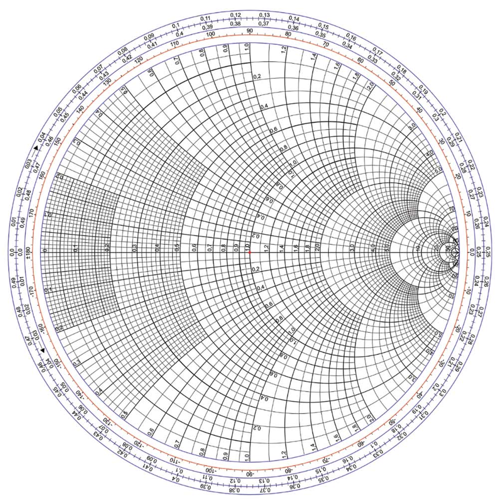
his is the second of the three articles devoted to the topic of a Smith Chart. The previous article, [1], introduced the concept of normalized load impedance and concluded with two equations describing the resistance and reactance circles. This article explains the creation of the resistance and reactance circles which are the basis of the graphical operations on the Smith Chart, like the one shown in Figure 1 [2].

Figure 1: Basic Smith Chart

The next two sections discuss the resistance and reactance circles and are based on the material presented in [3].

Relevant Background

Figure 2 shows a typical model of a lossless transmission line.

Model 1 - the source located at z = 0 and the load at z = L

Figure 2: Typical model of a lossless transmission line

With this transmission line we associate the load reflection coefficient,

, given by

(1.1)

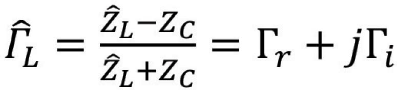
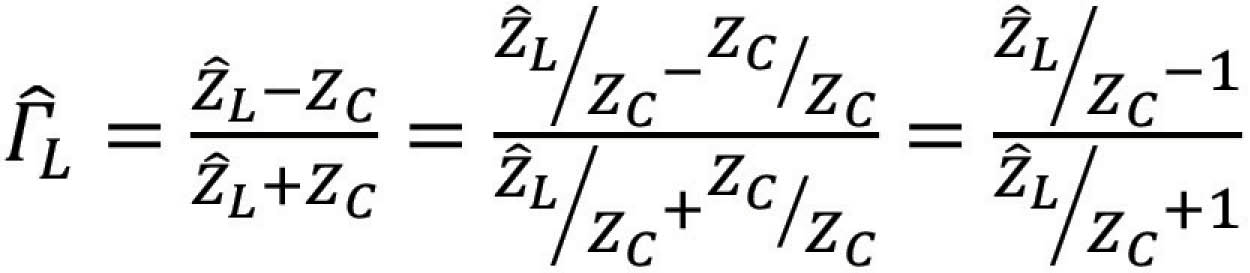
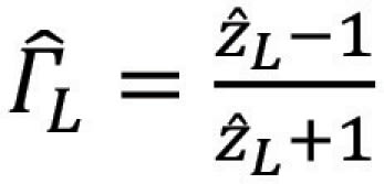
This load reflection coefficient can be expressed in terms of the normalized load impedance by dividing the numerator and denominator by the characteristic impedance of the line, Z_C.

(1.2)

(1.3)

where

(1.4)

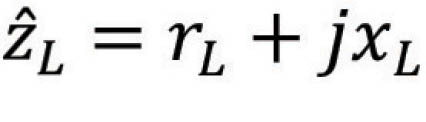
is the normalized load impedance, r_L is the normalized load resistance and x_L is the normalized load reactance.

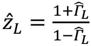
From Eq. (1.3) we can express the normalized load impedance in terms of the load reflection coefficient as

(1.5)

or, in terms of the real and imaginary parts as

(1.6)

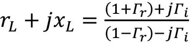
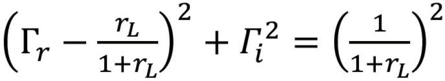
Equation (1.6) leads to the equation describing the resistance circle

(1.7)

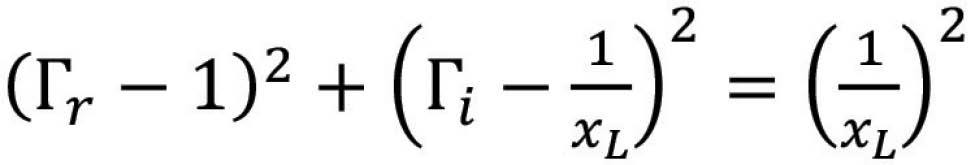
and another equation describing the reactance circle, [1],

(1.8)

Resistance Circles

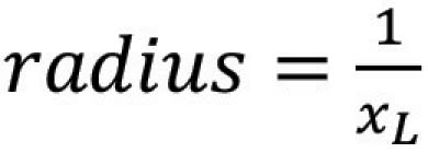
The resistance circle, described by Eq. (1.7) has a radius

(2.1)

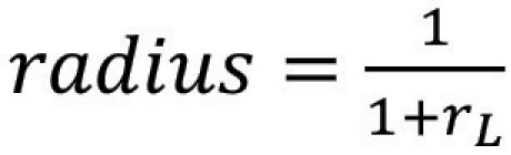
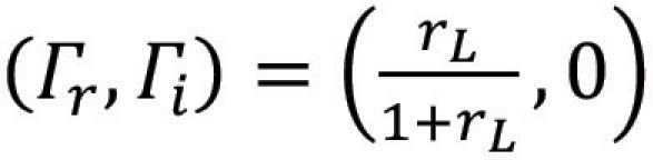
and is centered at

(2.2)

Let us calculate the radii and centers of the resistance circles for typical values of the normalized resistance r_L, [3]; this is shown in Table 1.

table graph of normalized resistance, radius, and center

Table 1: Radii and Centers of r-Circles

Figure 3 shows the plots of these circles on the complex Γ plane.

Model 2 - the load located at d = 0 and the source at d = L

Figure 3: Typical r-circles

Observations: All circles pass through the point (Γ_r, Γ_i) = (1,0). The largest circle is for r_L = 0, (which is the unit circle corresponding to). All circles lie within the bounds of Γ = 1 unit circle.

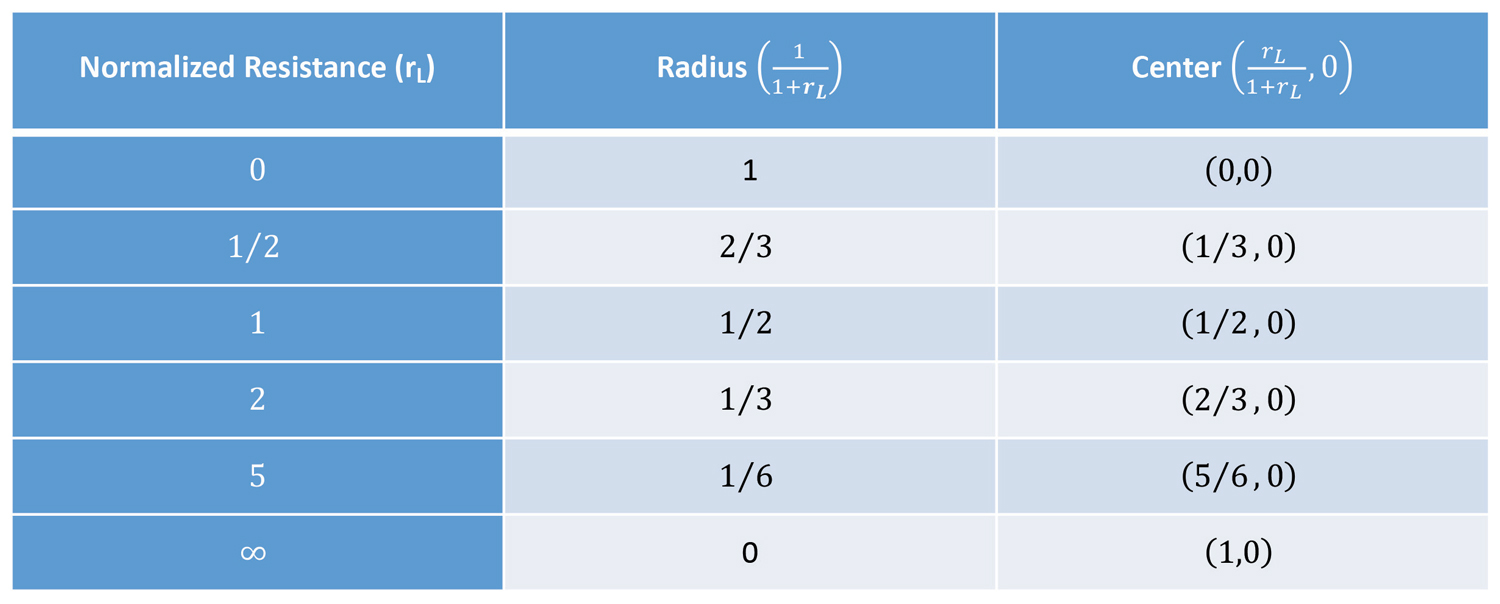
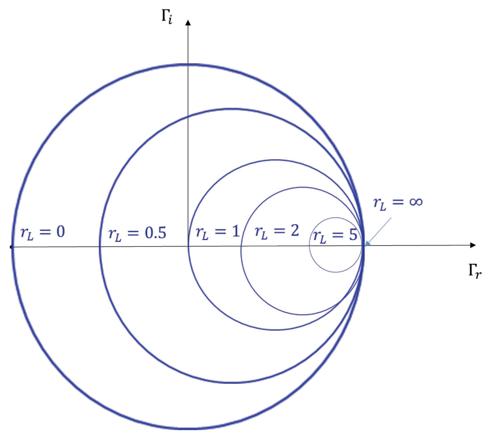
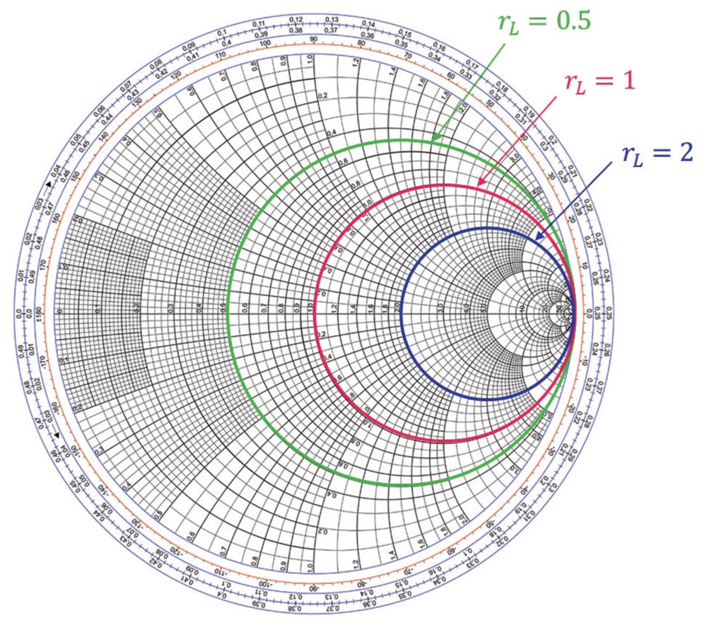
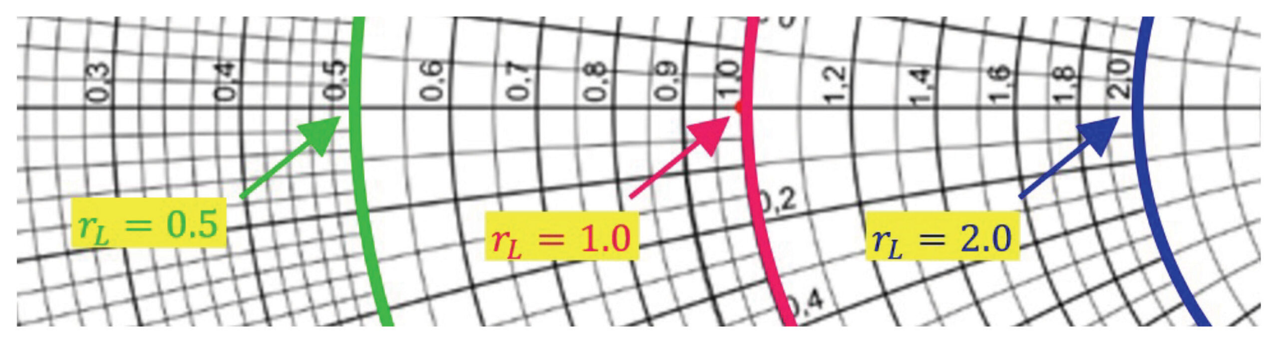
Let us identify some of these circles on the actual Smith Chart; this is shown in Figure 4.

Load reflection coefficient and the complex Γ plane

Figure 4: Selected r-circles on the Smith Chart

The values of the normalized resistances corresponding to these circles are shown on the horizontal axis (and other places) of the Smith Chart as shown in Figure 5.

Figure 5: Normalized resistance values on the Smith Chart

Reactance Circles

The reactance circle is described by

(3.1)

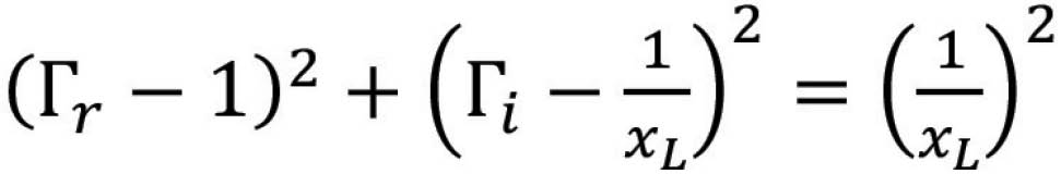
with the radius of

(3.2)

centered at

(3.3)

Let us calculate the radii and centers of the reactance circles for typical values of the normalized reactance x_L, [3].Note that unlike the normalized resistance (which is always non-negative), the normalized reactance can be positive (inductive load) or negative (capacitive load). Thus, Eq. (3.1) represents two families of circles, as shown in Table 2 and Figure 6.

Table 2: Radii and Centers of x-Circles

Figure 6: Typical x-circles

Of interest to us is the part of a given reactance circle that falls within the bounds of

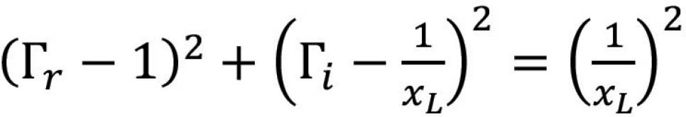
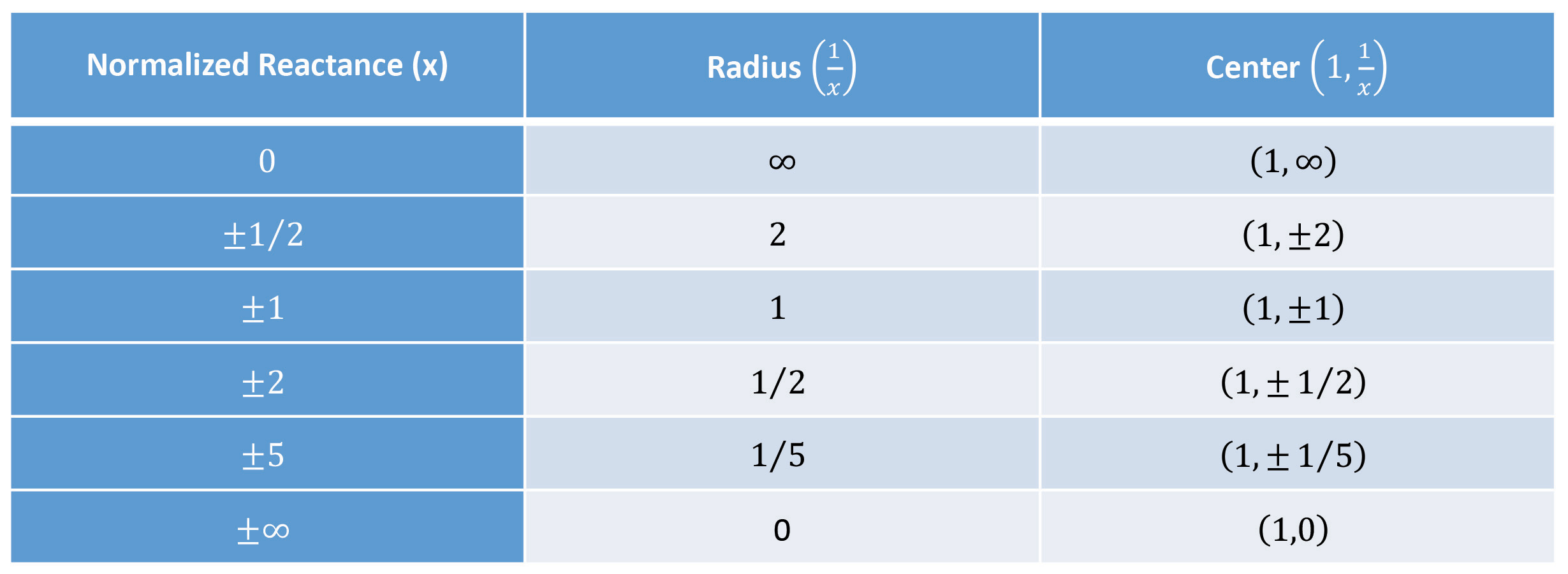
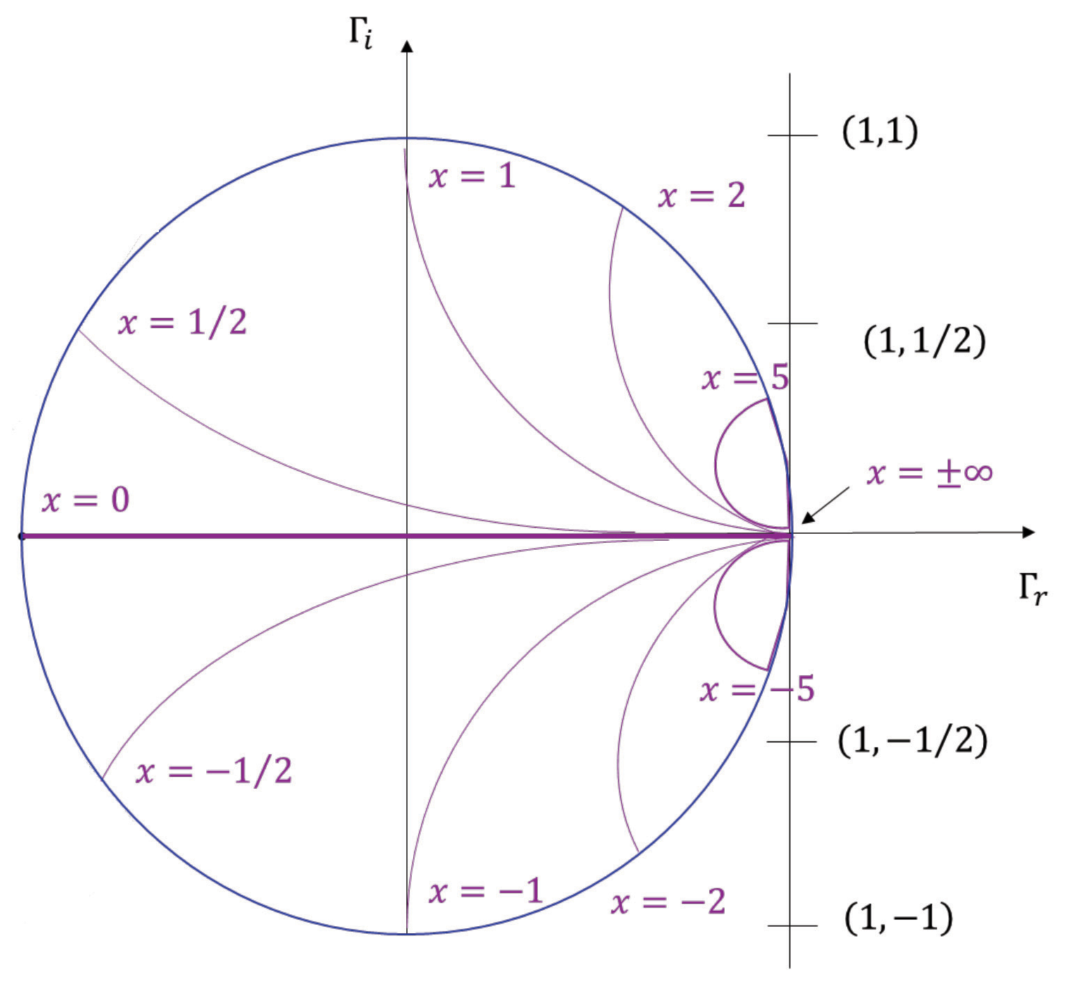
Γ = 1 unit circle.

Observations: The centers of all the reactance circles lie on the vertical Γ_r = 1 line. All reactance circles also pass through the (Γ_r, Γ_i) = (1,0) point (just like the r_L circles).

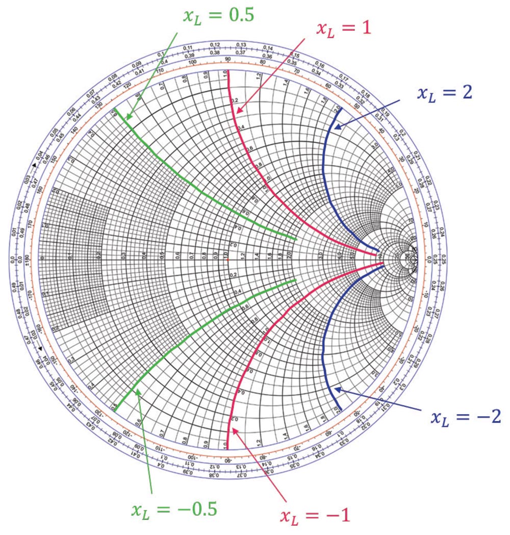
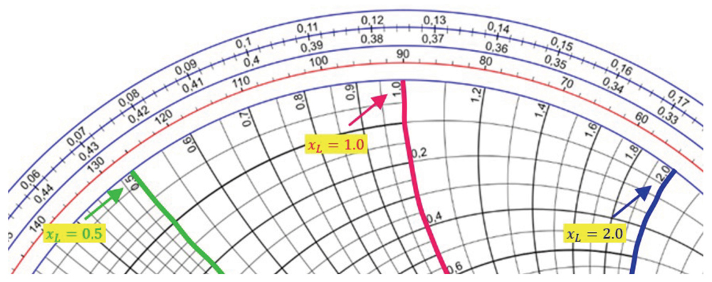
Let us identify some of these partial circles on the actual Smith Chart; this is shown in Figure 7.

Figure 7: Parts of the selected x-circles on the Smith Chart

The values of the normalized reactances corresponding to these partial circles are shown on the perimeter circle (and other places) of the Smith Chart, as shown in Figure 8.

Figure 8: Normalized reactance values on the Smith Chart

When we superimpose the resistance and reactance circles onto each other, we obtain Smith Chart shown in Figure 1.

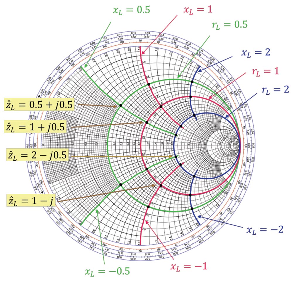
The intersection of any r-circle with any x-circle corresponds to a normalized load impedance, as shown in Figure 9.

Figure 9: Normalized load impedance on the Smith Chart

The next article will discuss the use of the Smith Chart in determining the input impedance to the transmission line at a given distance from the source or the load.

References

Adamczyk, B., “Smith Chart and Input Impedance to Transmission Line – Part 1: Basic Concepts,” In Compliance Magazine, April 2023.
https://upload.wikimedia.org/wikipedia/commons/7/7a/Smith_chart_gen.svg
Fawwaz Ulaby and Umberto Ravaioli, “Fundamentals of Applied Electromagnetics,” Pearson Education Limited, 7^th Ed., 2015.

Share this story:

Dr. Bogdan Adamczyk is professor and director of the EMC Center at Grand Valley State University (http://www.gvsu.edu/emccenter) where he regularly teaches EMC certificate courses for industry. He is an iNARTE certified EMC Master Design Engineer. Prof. Adamczyk is the author of the textbook “Foundations of Electromagnetic Compatibility with Practical Applications” (Wiley, 2017) and the upcoming textbook “Principles of Electromagnetic Compatibility with Laboratory Exercises” (Wiley 2023). He can be reached at adamczyb@gvsu.edu.

Back to Issue