his article discusses the impact of a shunt inductive discontinuity along the line as well as the effect of feeding two transmission lines in parallel. The analytical results are verified through the HyperLynx simulations and laboratory measurements.
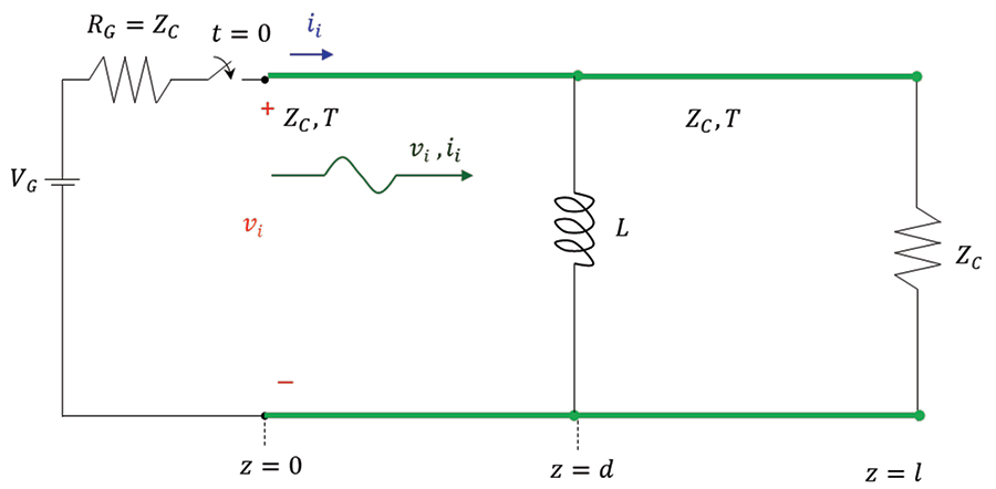
When the switch closes at t = 0, a wave originates at z = 0, [1], with
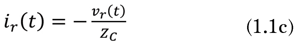
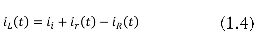
The current iR (t) can be expressed as
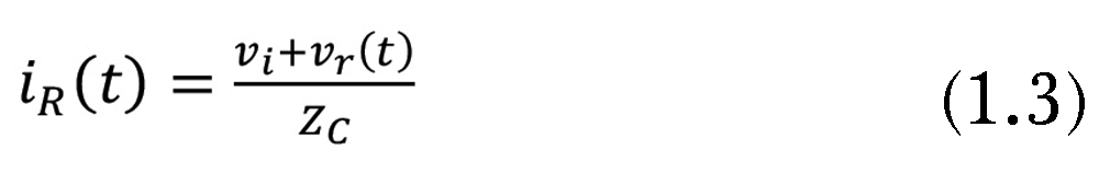
or
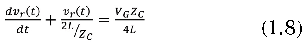
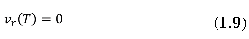
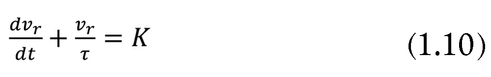
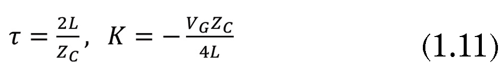
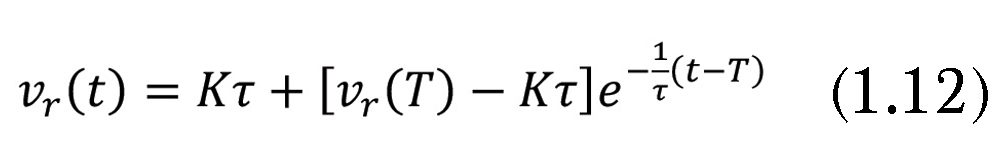
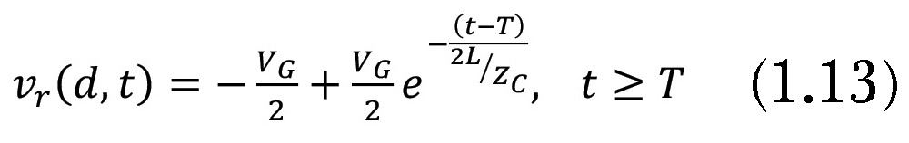
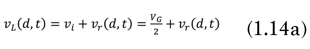
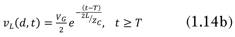
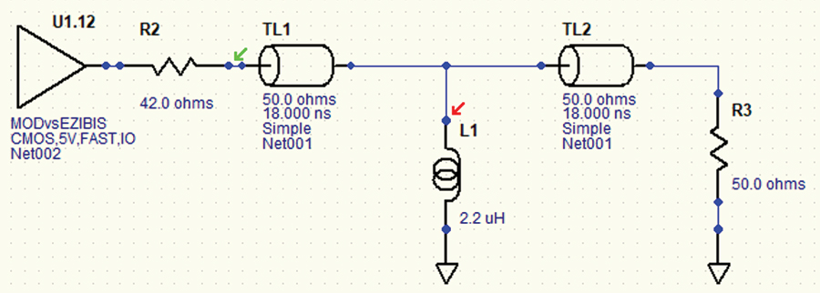
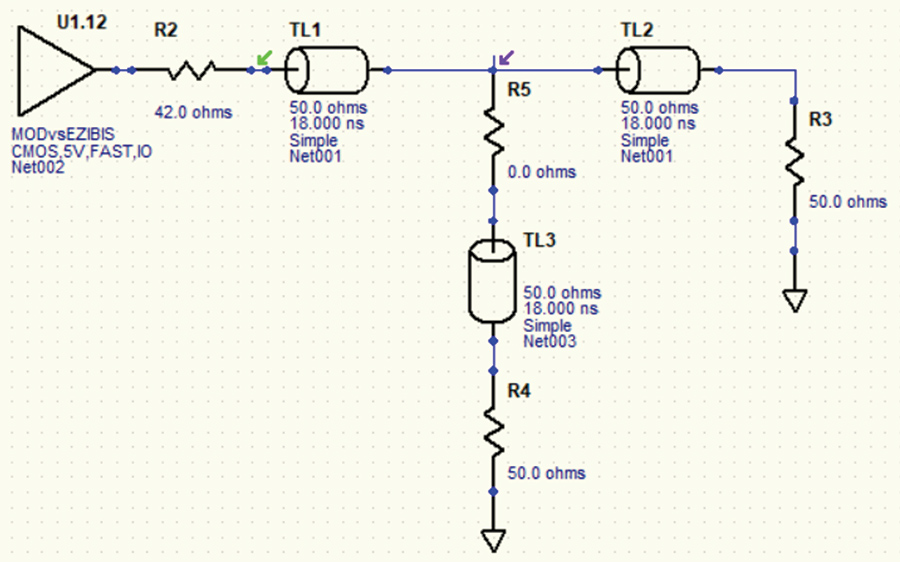
Figure 1.3 shows the HyperLynx schematic of the transmission line with an inductive discontinuity.
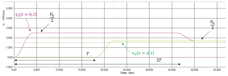
Note that the simulation results verify the analytical results.
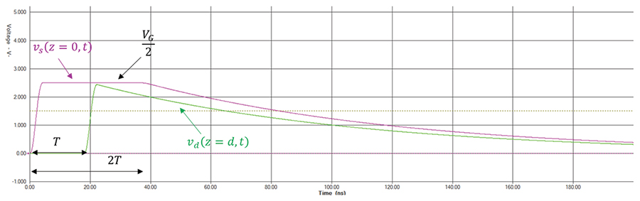
Figure 1.4: Inductive discontinuity – Voltages at the source (z = 0 ) and the load (z = d )
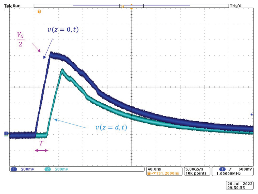
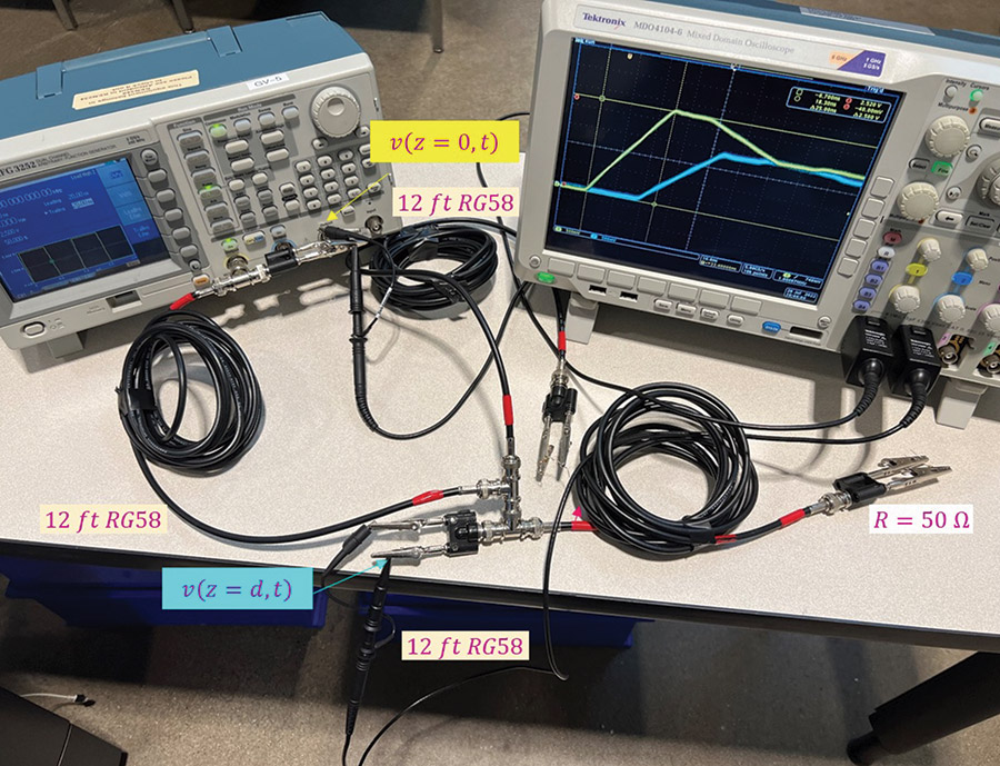
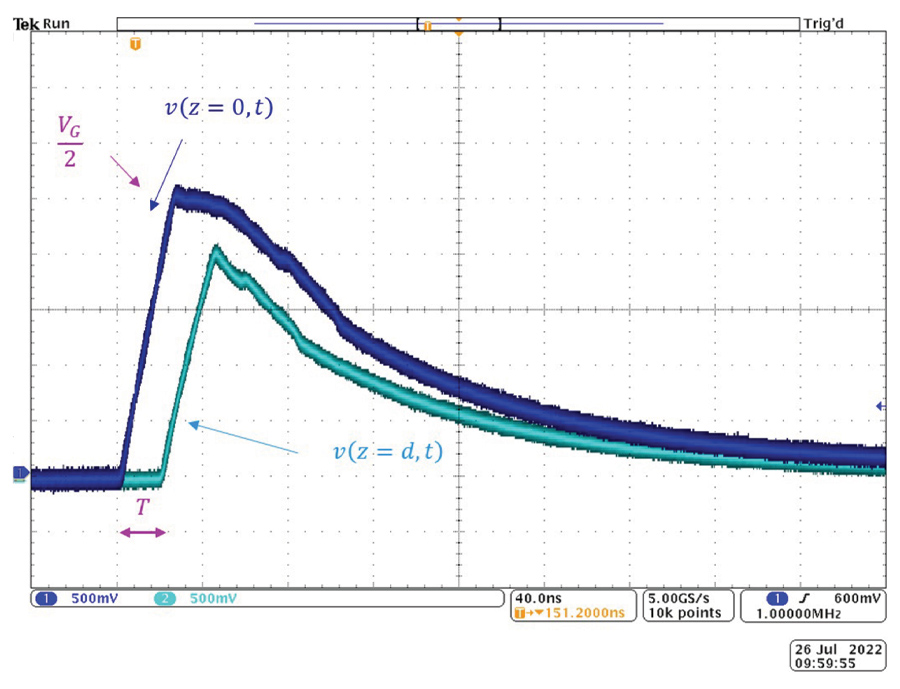
Note that the measurement results verify the simulation and analytical results.
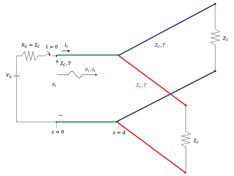
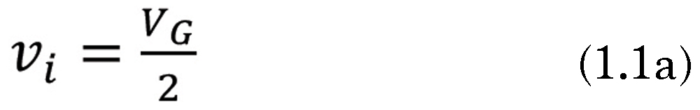
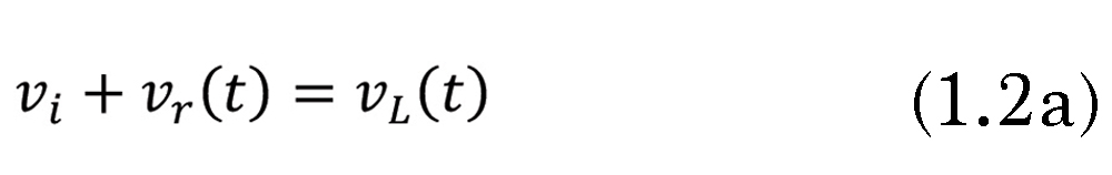
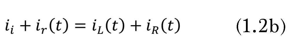
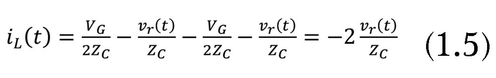
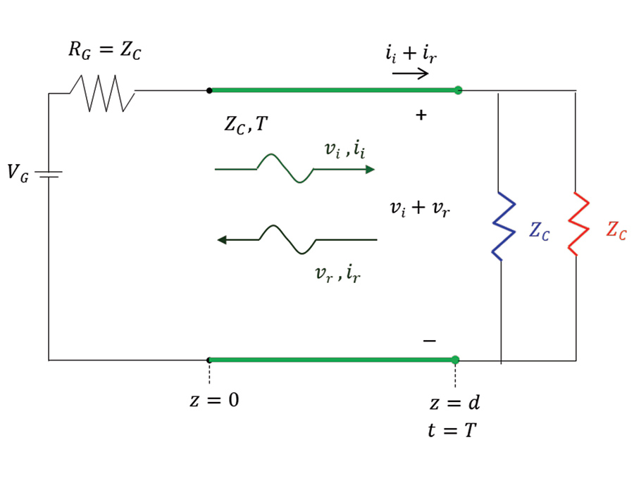
When the switch closes at t = 0, a wave originates at z = 0 and travels towards the discontinuity. The transmission lines immediately to the right of the discontinuity look to the circuit on the left of the discontinuity like two resistances in parallel. Their values are equal to the corresponding values of their characteristic impedances. When the incident wave arrives at the discontinuity (at the time t = T), the reflected wave, vr and ir, is created, and we have a situation depicted in Figure 2.2.
References
- Adamczyk, B., “Transmission Line Reflections at a Resistive Load,” In Compliance Magazine, January 2017.
- Adamczyk, B., Foundations of Electromagnetic Compatibility with Practical Applications, Wiley, 2017.
- Adamczyk, B., “Transmission Line Reflections at a Shunt Resistive and Reactive Discontinuity Along the Line,” In Compliance Magazine, October 2022.
