EMC concepts explained
Analysis of Transmission Lines in Sinusoidal Steady State
Different Circuit Models and Their Applications: Part 2
T

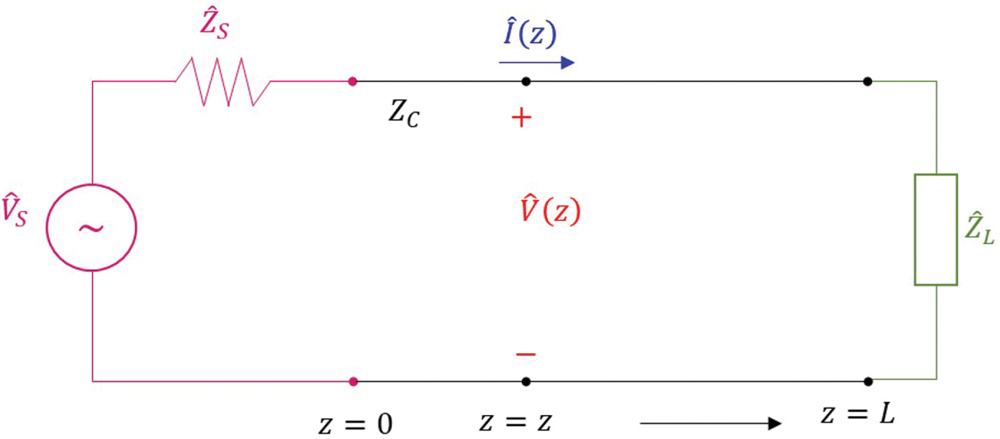
his is the second of three articles discussing four different circuit models of transmission lines in sinusoidal steady state. In Part 1 [1], Model 1 and Model 2 were presented. In this article, we focus on Model 3. Model 3 is mathematically most expedient for evaluating the values of the minima and maxima of standing waves. The locations of the minima and maxima of standing waves are determined using Model 4.

Transmission Line Model 3
To present Model 3, it is helpful to recall Model 1, shown in Figure 1.
Transmission line circuit – Model 1
Figure 1: Transmission line circuit – Model 1
In Model 1, we are moving away from the source located at z = 0 towards the load located at z = L. Model 3, shown in Figure 2, is obtained from Model 1.
Transmission line circuit – Model 3
Figure 2: Transmission line circuit – Model 3
In this Model we are moving away from the source to the load, just like we did in Model 1. But in Model 3, the source is located at z = –L while the load is located at z = 0.

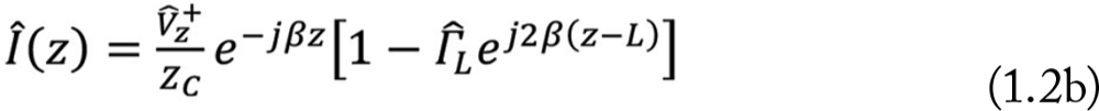
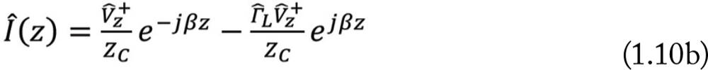
In both models, the voltage and current at any location z, away from the source, are given by the same equations:

equation
equation
These equations describe the voltage and current along the line, regardless of the value of z, assigned to the location of the source. We can place that location at any convenient point along the line, depending on what phenomenon we want to investigate. In computing the value of the voltage maxima and minima, the source location chosen in Model 3 is the most convenient.

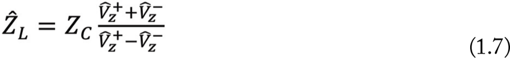
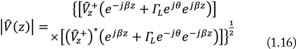
It is important to discern which equations are the same and which are different in both models. In Model 1, the voltage and current at any location z, away from the source, was expressed in terms of the load reflection coefficient as [1],

equation
equation
where 
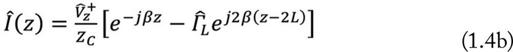
L is the load reflection coefficient. These equations can be written in an alternative way.
equation
equation
or
equation
equation
Equations (1.2), (1.3), and (1.4), valid for Model 1, describe voltage and current at any location z away from the source when the source is located at z = 0 and the load is located at z = L. As we shall see, the corresponding set of equations for Model 3 is different.

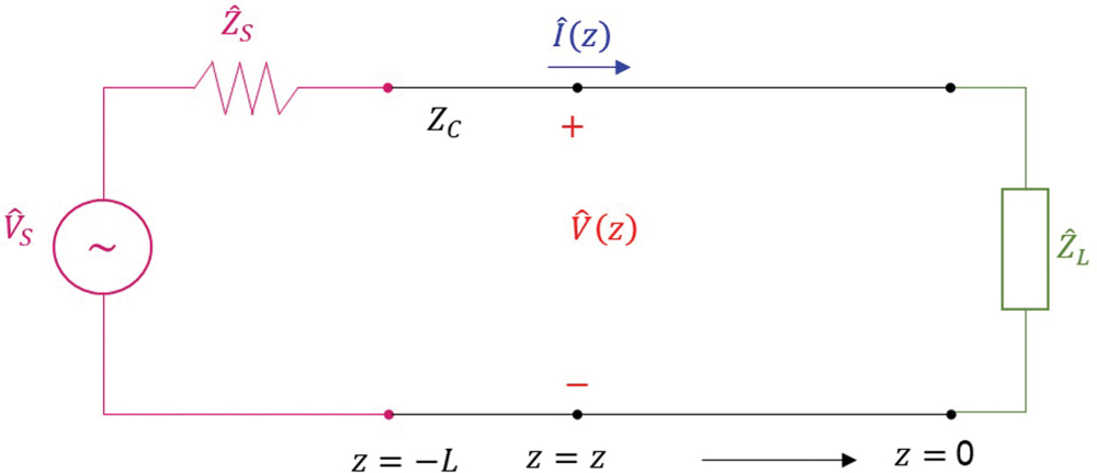
In Model 3, with the choice of the z = 0 location at the load, the following equation must be satisfied:

equation
From Eqns. (1.1), valid for both models, we get
equation
equation
Utilizing Eqns. (1.6) in Eq. (1.5), we have
equation
leading to
equation
or
equation
Using Eq. (1.9) in Eqns. (1.1), we get
equation
equation
or
equation
equation
Note that Eqns. (1.11), valid for Model 3, are different from Eqns. (1.4), valid for Model 1. We will use Eqn. (1.11a) to determine the expression for the voltage magnitude and, subsequently, its maximum and minimum. Towards this end, let’s express the complex load reflection coefficient in terms of its magnitude and angle as
equation
Utilizing Eq. (1.12) in Eq. (1.11a) we get
equation
The magnitude of a complex voltage in Eq. (1.13) can be obtained from
equation
where the superscript * denotes a complex conjugate. Thus,
equation
or
equation
Multiplying out and simplifying, we have
equation
Utilizing Euler’s formula for a cosine, we arrive at the expression for the magnitude of the voltage at any location z away from the source as
equation
when the source is located at z = –L and the load is located at z = 0, (Model 3).

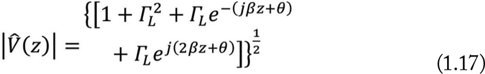
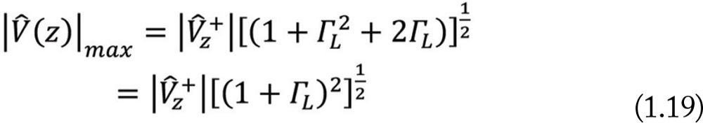
The maximum magnitude of the voltage in Eq. (1.18) occurs when the cosine function equals 1. Thus,

equation
or
equation
The minimum magnitude of the voltage in Eq. (1.18) occurs when the cosine function equals -1. Thus,
equation
or
equation
Additionally, Eqns. (1.20) and (1.22) provide an alternative and convenient way of calculating the voltage standing wave ratio (VSWR), as
equation
Transmission Line Model 4
Model 4 is shown in Figure 3. In Model 4, we are moving away from the load located at d = 0 towards the source located at d = L.
Transmission line circuit – Model 4
Figure 3: Transmission line circuit – Model 4
Model 4 is obtained from Model 3 by simply relating the distance variables according to
equation
Using Eq. (1.24), in Eq. (1.18), the magnitude of the voltage at any location d away from the load becomes
equation
where
equation
Equation (1.25) can be rewritten as
equation
Since cosine is an even function, Eq. (1.27) becomes
equation
The next article will utilize Model 4 and Eq. 1.27 to determine the locations of the voltage maxima and minima in terms of the distance d away from the load.
References
Adamczyk, B., “‘Analysis of Transmission Lines in Sinusoidal Steady State – Different Circuit Models and Their Applications: Part 1,” In Compliance Magazine, October 2024.
Share this story:
Bogdan Adamczyk headshot
Dr. Bogdan Adamczyk is professor and director of the EMC Center at Grand Valley State University (http://www.gvsu.edu/emccenter) where he performs EMC educational research and regularly teaches EM/EMC courses and EMC certificate courses for industry. He is an iNARTE-certified EMC Master Design Engineer. He is the author of two textbooks, “Foundations of Electromagnetic Compatibility with Practical Applications” (Wiley, 2017) and “Principles of Electromagnetic Compatibility: Laboratory Exercises and Lectures” (Wiley, 2024). He has been writing “EMC Concepts Explained” monthly since January 2017. He can be reached at adamczyb@gvsu.edu.