his article discusses the reflections on a transmission line at a shunt resistive and capacitive discontinuity along the line. The analytical results are verified through the HyperLynx simulations and laboratory measurements.
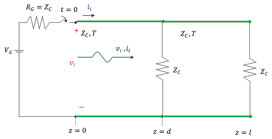
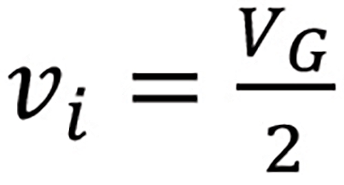
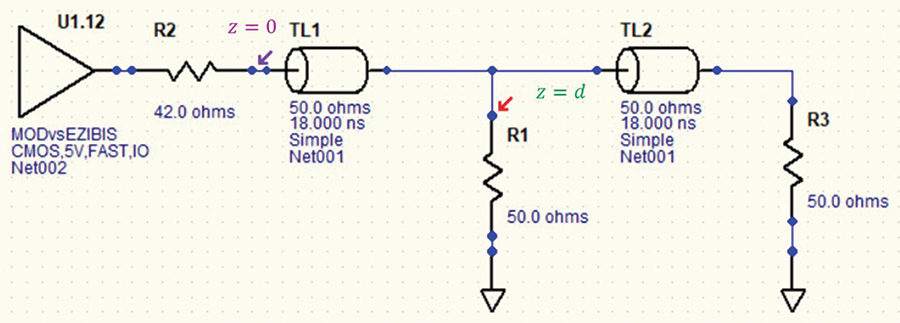
Note that the transmission line is matched at the source, and the resistive discontinuity and the load resistor values are equal to the characteristic impedance of the line.
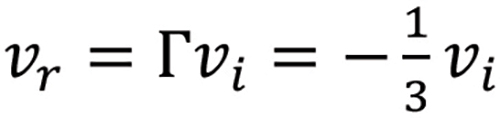
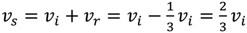
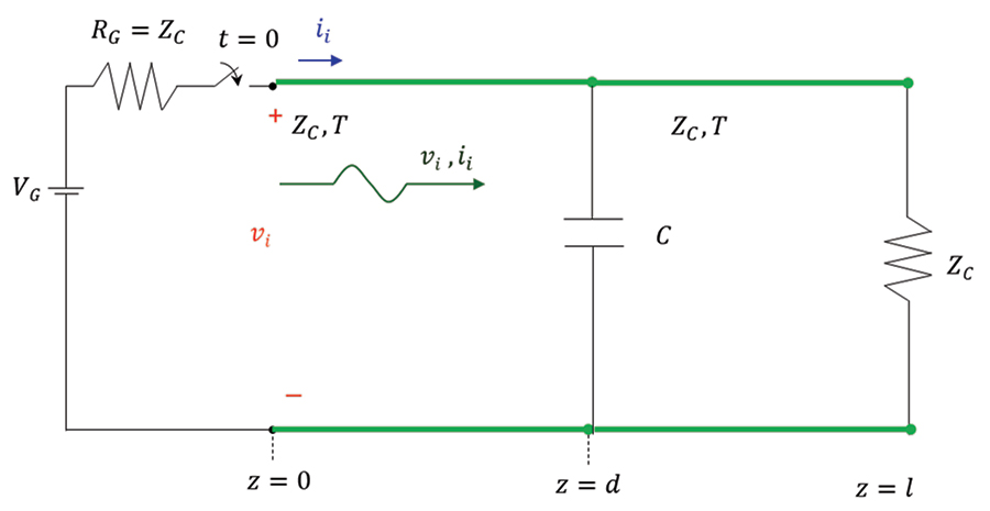
When the switch closes at t = 0, a wave originates at z = 0, [1], and travels towards the discontinuity. At the time, t = T this wave arrives at the discontinuity. The transmission line immediately to the right of the discontinuity looks to the circuit on the left of the discontinuity like a shunt resistance equal to the characteristic impedance of the right line [2].
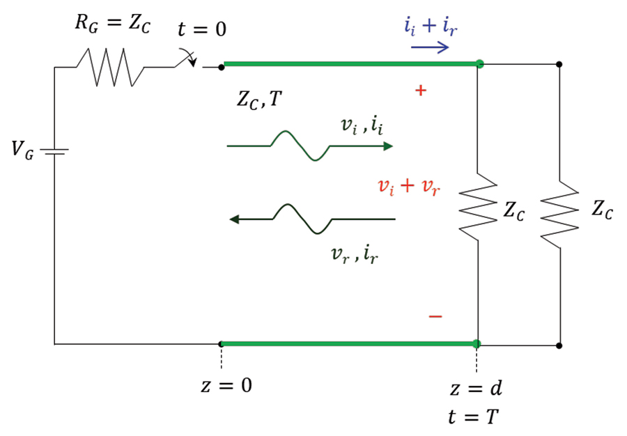
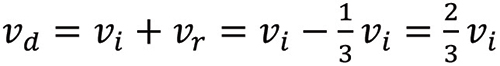
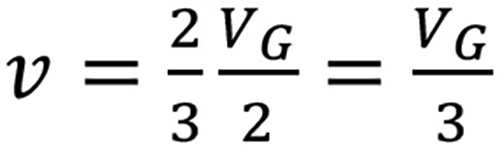
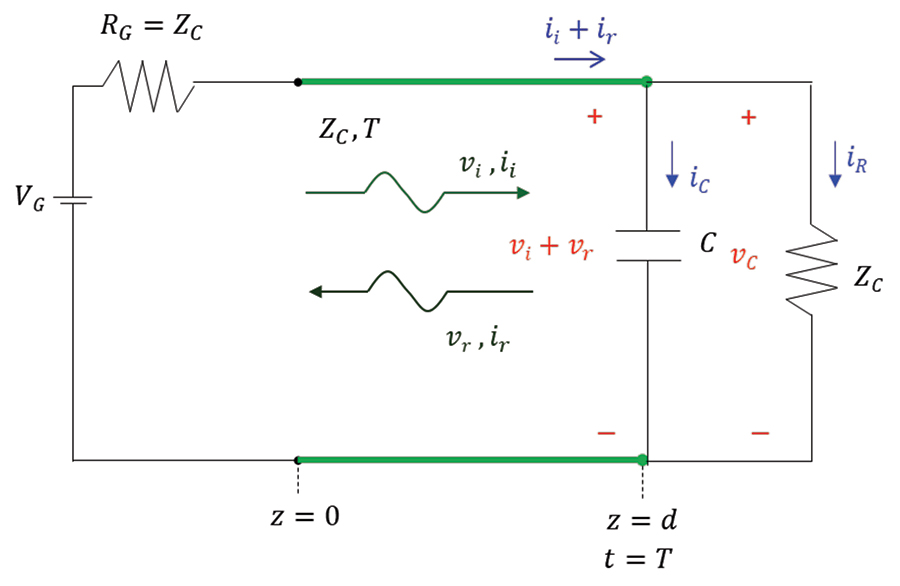
When this wave arrives at the discontinuity, at the time t = T, the reflected wave, vr and ir, is created, and we have a situation depicted in Figure 1.2.
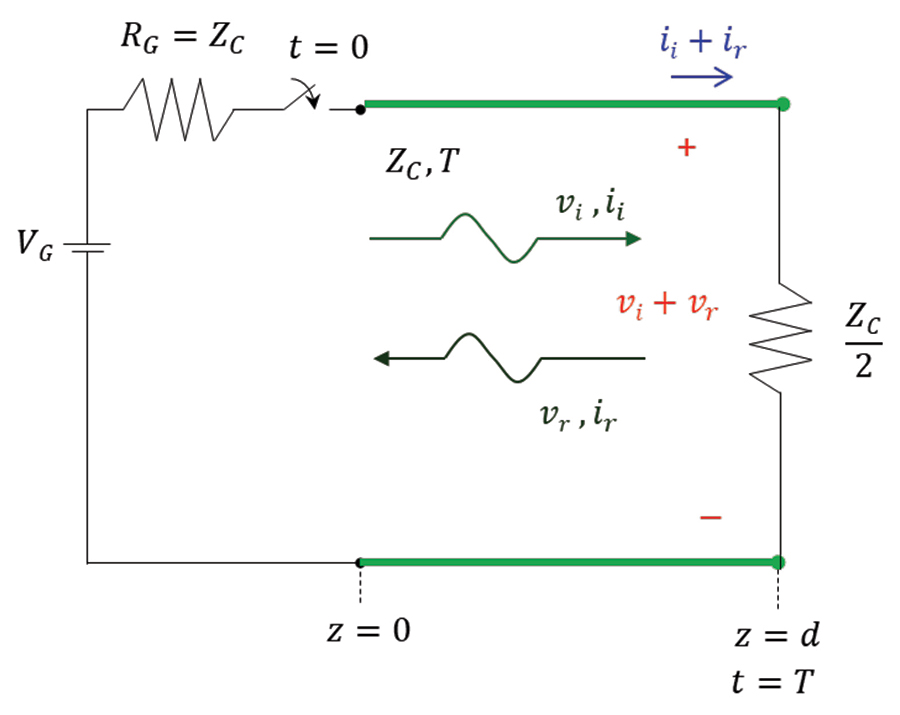
The circuit in Figure 1.2 is equivalent to the one shown in Figure 1.3.
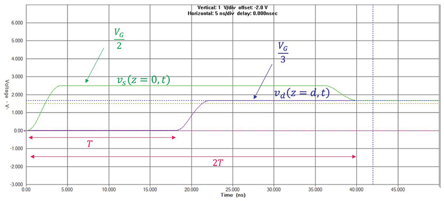
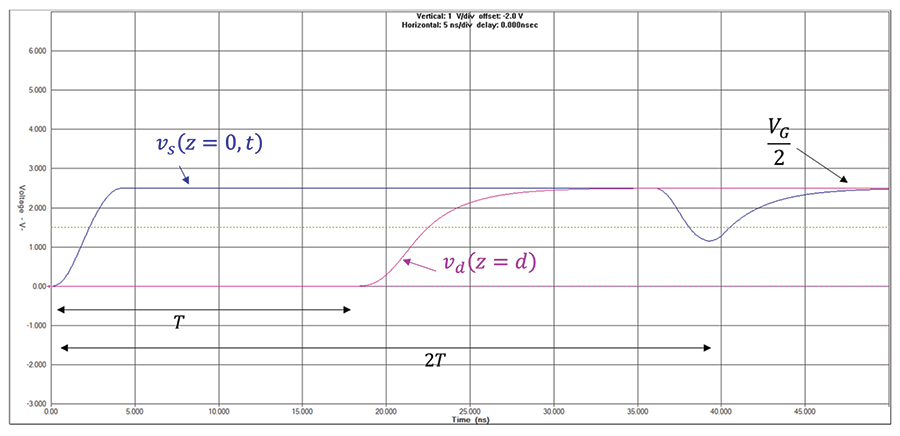
The simulation results are shown in Figure 1.5.
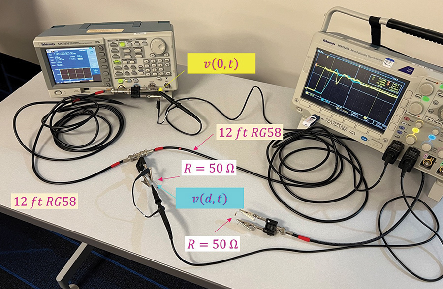
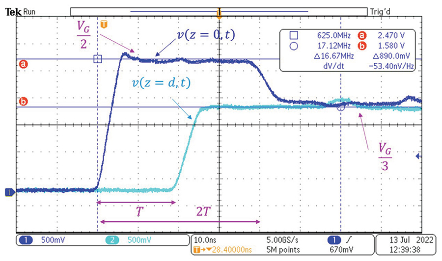
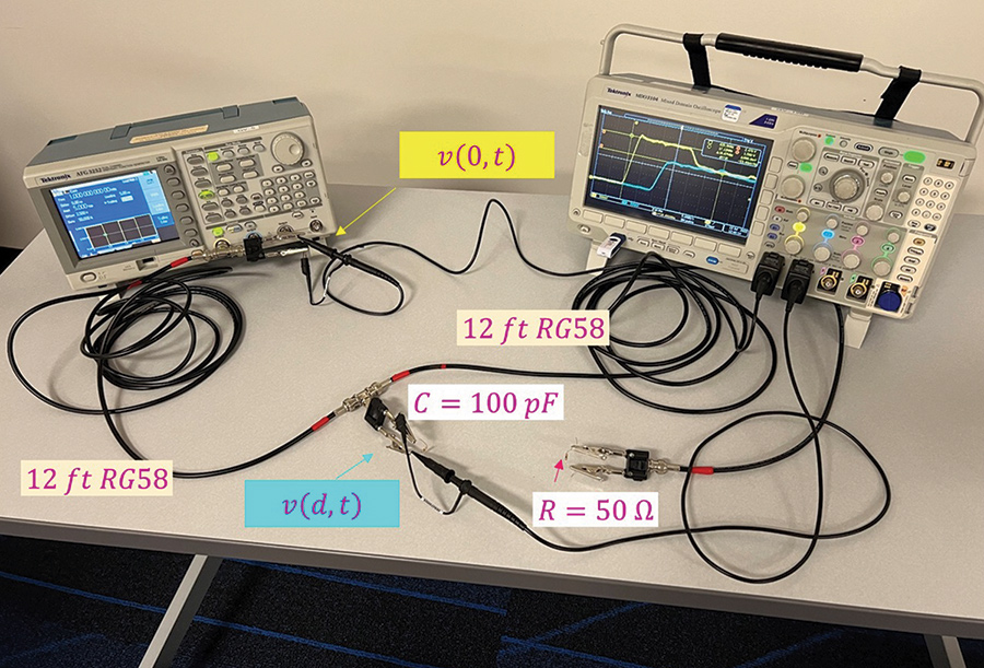
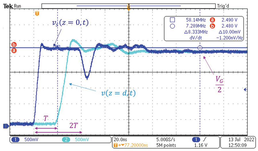
The measurement results are shown in Figure 1.7.
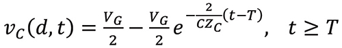
Note that the load resistor value is equal to the characteristic impedance of the transmission line; it is also assumed that the initial voltage across the capacitor is zero, vC (0–) = 0.
When the switch closes at t = 0, a wave originates at z = 0, [1], and travels towards the discontinuity.
The transmission line immediately to the right of the discontinuity looks to the circuit on the left of the discontinuity like a shunt resistance equal to the characteristic impedance of the right line [2]. When the incident wave arrives at the discontinuity (at the time t = T), the reflected wave, vr and ir, is created, and we have a situation depicted in Figure 2.2.
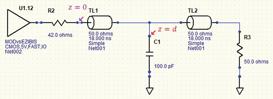
The simulation results are shown in Figure 2.4.
The measurement results are shown in Figure 2.6.
- Adamczyk, B., “Transmission Line Reflections at a Resistive Load,” In Compliance Magazine, January 2017.
- Adamczyk, B. Foundations of Electromagnetic Compatibility with Practical Applications, Wiley, 2017.
- Adamczyk, B., “Transmission Line Reflections at the RL and RC Loads,” In Compliance Magazine, January 2021.
