Correlation Between Insertion Loss and Input Impedance of EMC Filters

EMC concepts explained

Part 1: LC and CL Filters

his is the first article of a three-article series devoted to the correlation between the insertion loss and input impedance of passive EMC filters. In this article, we focus on LC and CL filters. Based on the analysis, simulation, and measurement results, it has been observed that the frequencies where the insertion losses of the filters are equal are also the frequencies where the input impedances are equal. These frequencies define the regions where one filter configuration outperforms the other (with respect to the insertion loss). To determine these regions analytically, we compare the input impedances of the two filters. Subsequent articles will focus on π and T filters and cascaded LC and CL configurations.

1. Insertion Loss Definition

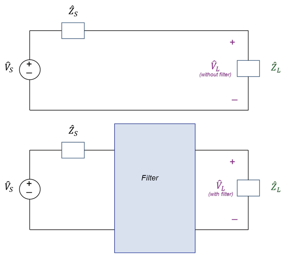
Consider the circuit shown in Figure 1.

Figure 1: Illustration of the insertion loss of a filter

Figure 2: Input impedance to the LC filter

Insertion loss of a filter can be defined as

(1a)

where V_L is the magnitude of the complex voltage _L . Since V_{L,without filter} > V_{L,with filter} the insertion loss defined by Eq. (1a) is a positive number in dB. The insertion loss could alternatively be defined as [1],

(1b)

In this case, the insertion loss in dB is the negative of the loss defined in Eq. (1b). We will use this definition when plotting the simulation results and comparing the simulation results to the VNA measurements.

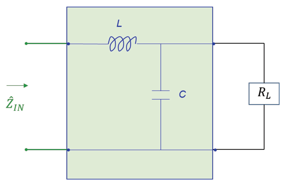
2. Input Impedance to the LC Filter

The input impedance,

_IN, to the LC filter is calculated from the circuit shown in Figure 2.

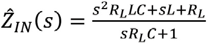
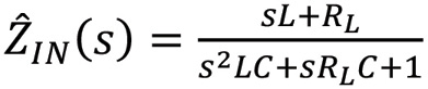
(2a)

(2b)

or, in terms of the frequency

(3a)

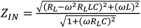
The magnitude of the input impedance is

(3b)

3. Input Impedance to the CL Filter

The input impedance,

_IN, to the CL filter is calculated from the circuit shown in Figure 3.

(4a)

(4b)

or, in terms of the frequency

(5a)

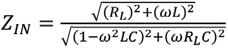
The magnitude of the input impedance is

(5b)

4. LC Filter vs. CL Filter – Input Impedance – Simulations and Calculations

Figure 4 shows the simulation circuit used for the comparison of input impedances.

Figure 3: Input impedance to the CL filter

Figure 4: Simulation circuit for comparison of input impedances

The simulation results are shown in Figure 5.

Note that the two input impedances are equal at the frequency of 1.0349 MHz. Figure 5 also shows the resonant frequency of the LC filter at 733.16 kHz. This result is confirmed by the calculations in Equation 6.

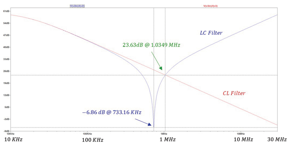
Figure 5: Simulation results: Input impedance – LC filter vs. CL filter

(6)

Next, let’s calculate the frequency at which the input impedances of the two filters are equal. Equating the expressions in equations (3b) and (5b) produces

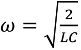
(7)

This equation can be solved for ω, [2], resulting in

(8a)

(8b)

Which agrees with the simulation result shown in Figure 5.

5. LC Filter vs. CL Filter – Insertion Loss – Simulations and Measurements

Figure 6 shows the simulation circuit used for the comparison of insertion losses.

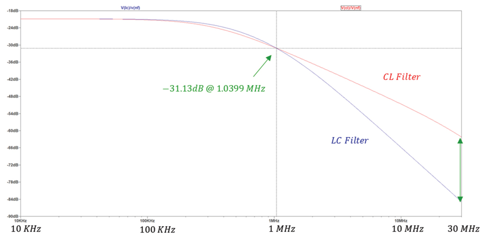
The simulation results are shown in Figure 7.

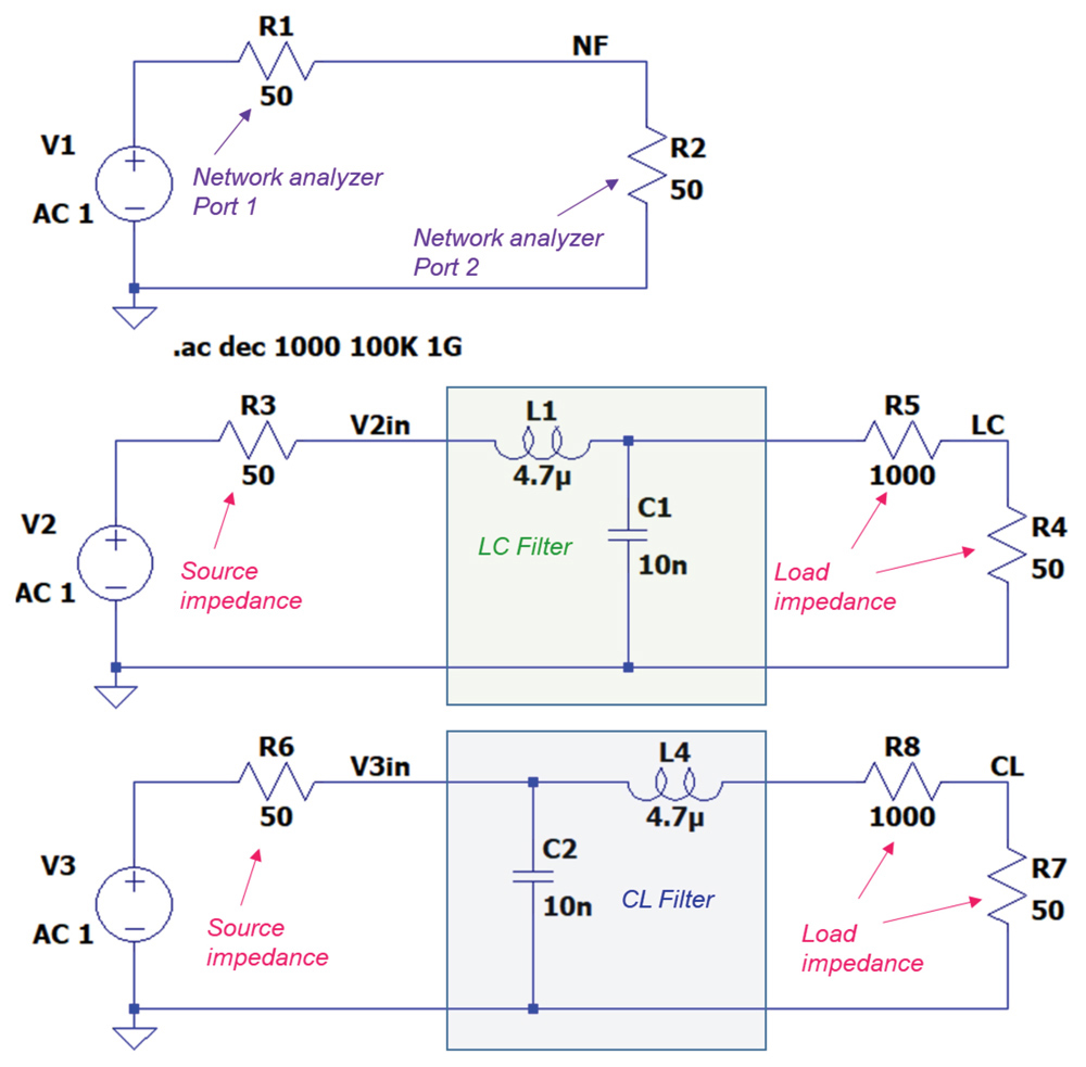
Figure 6: Simulation circuit for comparison of insertion losses

Figure 7: Simulation results: Insertion loss – LC filter vs. CL filter

The insertion losses of the two filters are equal at the frequency of 1.04 MHz. This is the same frequency at which the input impedances of the two filters were equal! Note that up to the frequency of 1.04 MHz the insertion loss of an CL filter is larger (in the absolute sense) than that of the LC filter. Beyond that frequency the insertion loss of the LC filter is larger. This means that the LC filter is more effective than the CL filter beyond the frequency of 1.04 MHz.

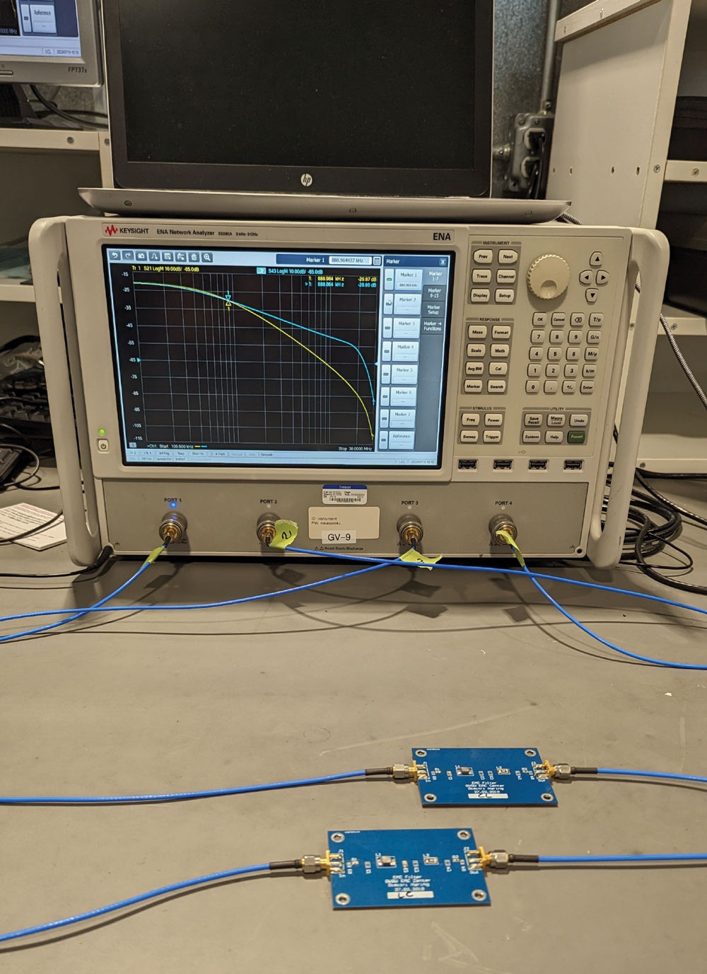
Figure 8: Measurement setup: Insertion loss – LC filter vs. CL filter

We have arrived at a very important observation: once the filter components values L and C are chosen, we can determine the frequency at which the insertion losses of LC and CL filters are equal. This is the frequency at which the input impedances are equal and given by Eq. (8b).

To verify the simulations results of the insertion loss the measurement setup shown in Figure 8 was used.

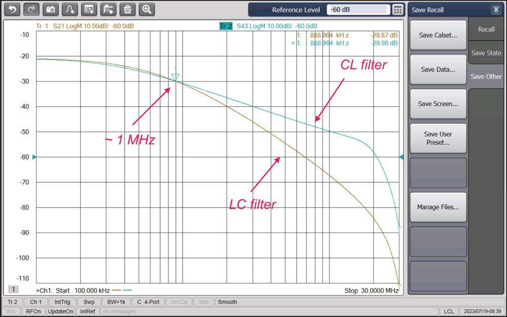
Figure 9: Measurement results: Insertion loss – LC filter vs. CL filter

The measurement results are shown in Figure 9.

Note that the measurement results agree with the calculated and simulated results.

References

Bogdan Adamczyk and Dimitri Haring, “EMC Filters Comparison Part I: CL and LC Filters,” In Compliance Magazine, December 2019.
Bogdan Adamczyk, Principles of Electromagnetic Compatibility: Laboratory Exercises with Lectures, Wiley, 2024.

Share this story:

Dr. Bogdan Adamczyk is professor and director of the EMC Center at Grand Valley State University (http://www.gvsu.edu/emccenter) where he regularly teaches EMC certificate courses for industry. He is an iNARTE certified EMC Master Design Engineer. Prof. Adamczyk is the author of the textbook “Foundations of Electromagnetic Compatibility with Practical Applications” (Wiley, 2017) and the upcoming textbook “Principles of Electromagnetic Compatibility with Laboratory Exercises” (Wiley 2023). He can be reached at adamczyb@gvsu.edu.

Jake Timmerman is an EMC Engineer at E3 Compliance, which specializes in EMC & SIPI design, simulation, pre-compliance testing, and diagnostics. He received his B.S.E in Electrical Engineering from Grand Valley State University. Jake participates in the industrial collaboration with GVSU at the EMC Center. He can be reached at jacob.timmerman@e3compliance.com.

Back to Issue