

n Part 2 of this series [1], we introduced you to radiated emissions pre-compliance testing for commercial, industrial, and medical products. Here, we’ll cover the differences in making the measurements for automotive modules and military products. In the next part of this series, we’ll describe some pre-compliance software that will help automate these manual measurements.
Readers will want to refer to the general test equipment setups, gain and loss calculations, and test procedures described in Parts 1 and 2. [1, 2] Additional details may be found in References 3 and 4.
Most automotive and military EMC tests for components, modules, or smaller products are tested in a similar environment to where the product is to be installed. This is a major difference in consumer testing in that we’re less concerned about interference to established communications and broadcast (TV, radio, aircraft, land mobile, and mobile phone) and more concerned with how a product behaves in the environment it’s designed for (automotive cockpits, military vehicles, shipboard, spacecraft, and military or commercial aircraft.
In other words, we’re not so much interested in far-field emissions or interference (3m or 10m test distance) but more interested in whether a product is compatible with other equipment installed close by and located more in the near field (1m test distance).
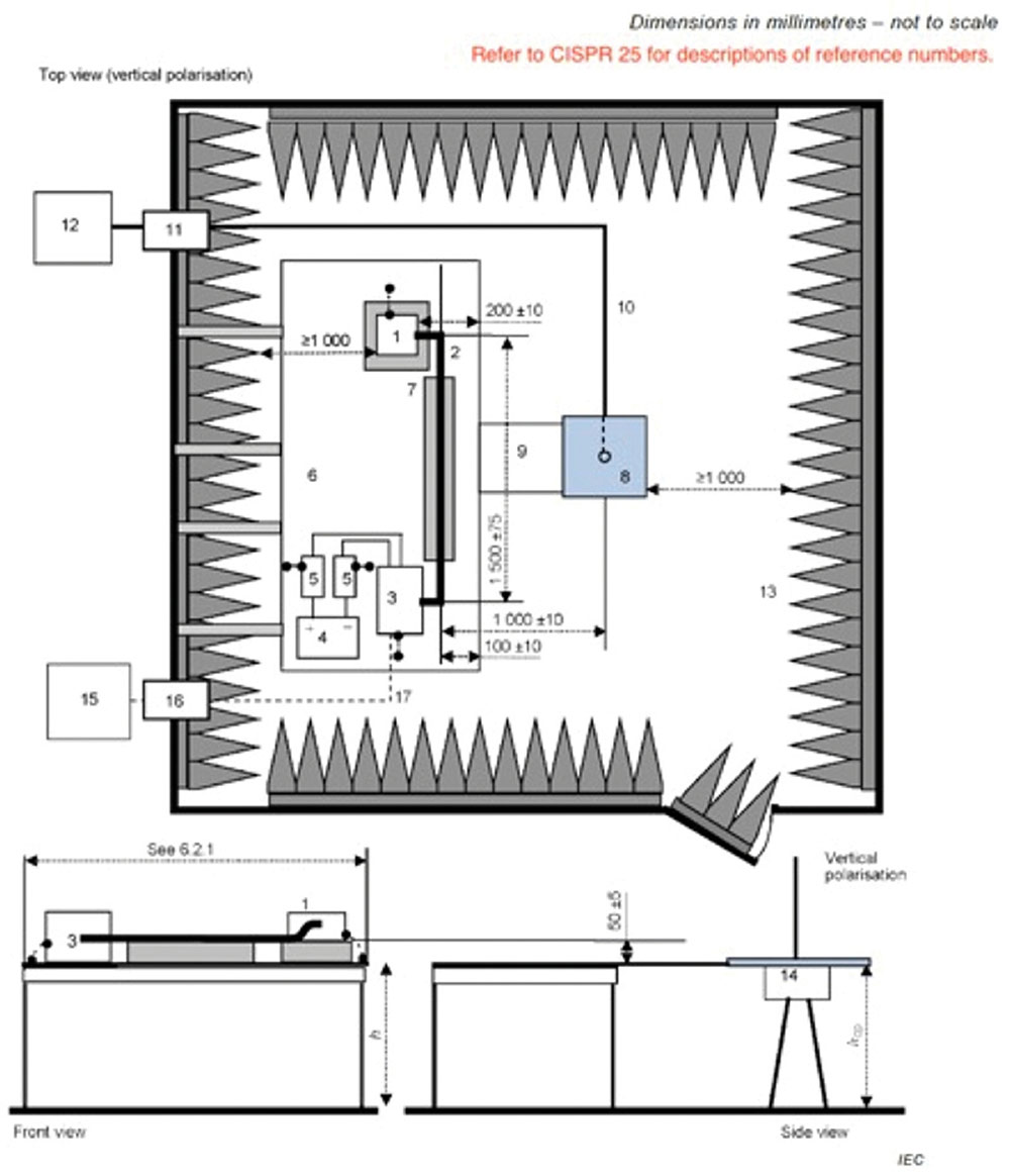
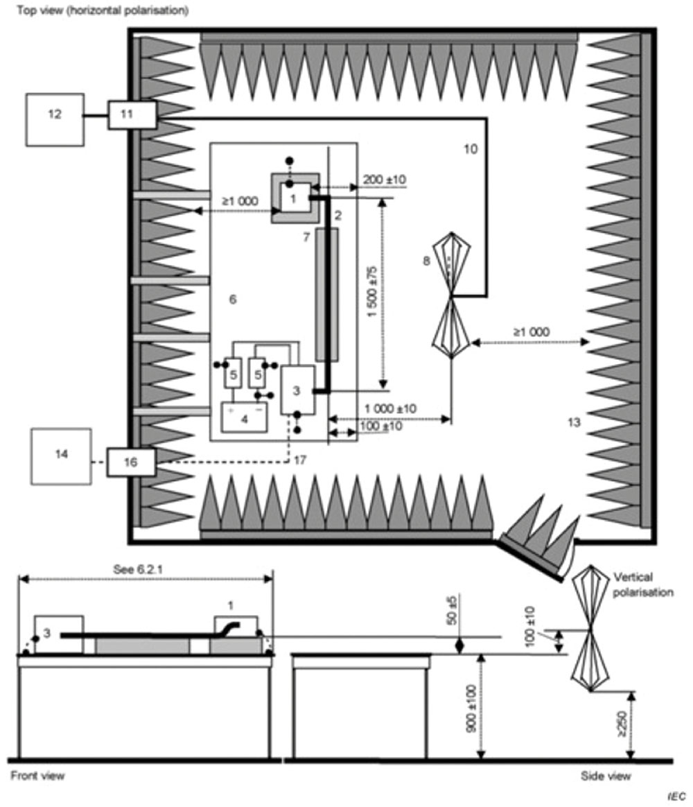
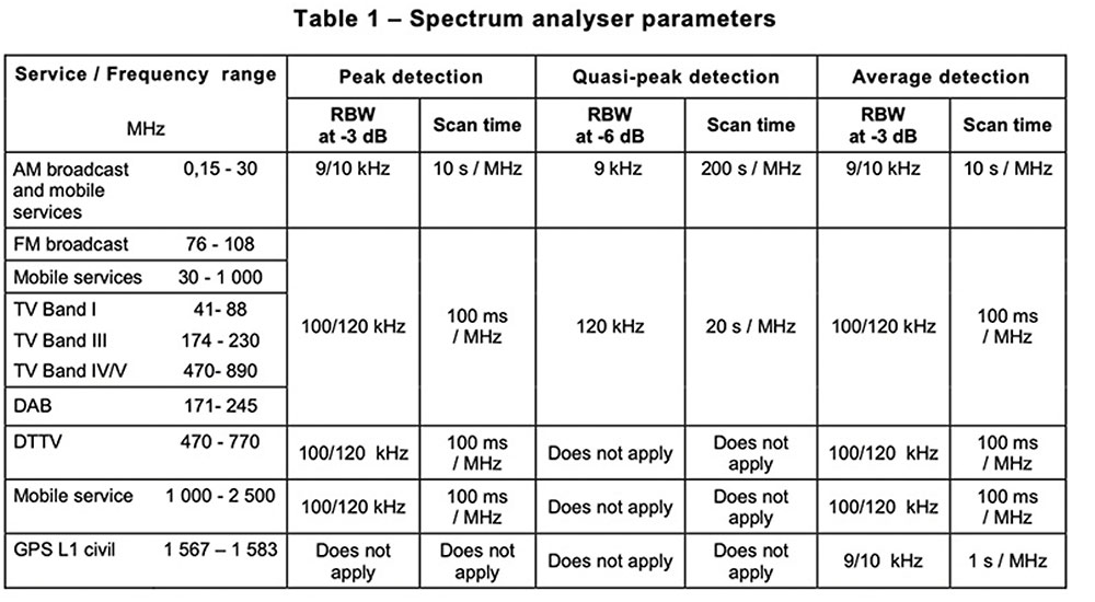
The resolution bandwidth setting of the spectrum analyzer depends on the frequency bands being tested. For radiated emissions in the range of 30 to 2500 MHz, this should be set to 100 or 120 kHz. The video bandwidth should be set at least three times the resolution bandwidth. A broadband preamplifier may be used to achieve at least a 6-dB noise floor below the test limits. There are separate limits for peak, quasi-peak, and average detection. For details, refer to Figure 3 and CISPR 25 (or the equivalent Euro Norm, EN 55025).
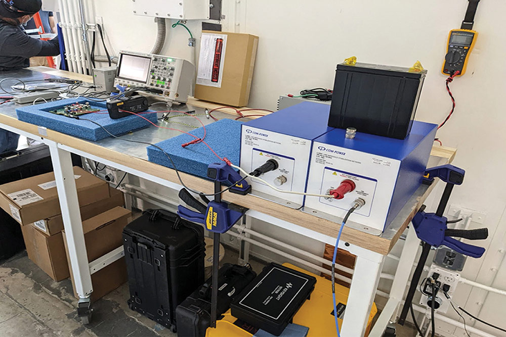
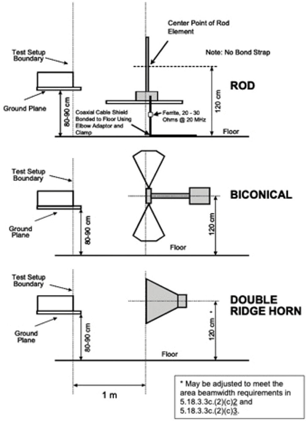
Figures 4 and 5 show typical CISPR 25 test setups for automotive module testing.
Set up your spectrum analyzer the same way as in CISPR 25 above. The resolution bandwidths should be set according to Table II in MIL‑STD-461 (Figure 7 on page 20). For radiated emissions, the RBW will be set between 10 kHz and 1 MHz, depending on the band scanned. The standard calls for peak detection. These bandwidths are specified at the 6 dB down points for the overall selectivity curve of the receivers.
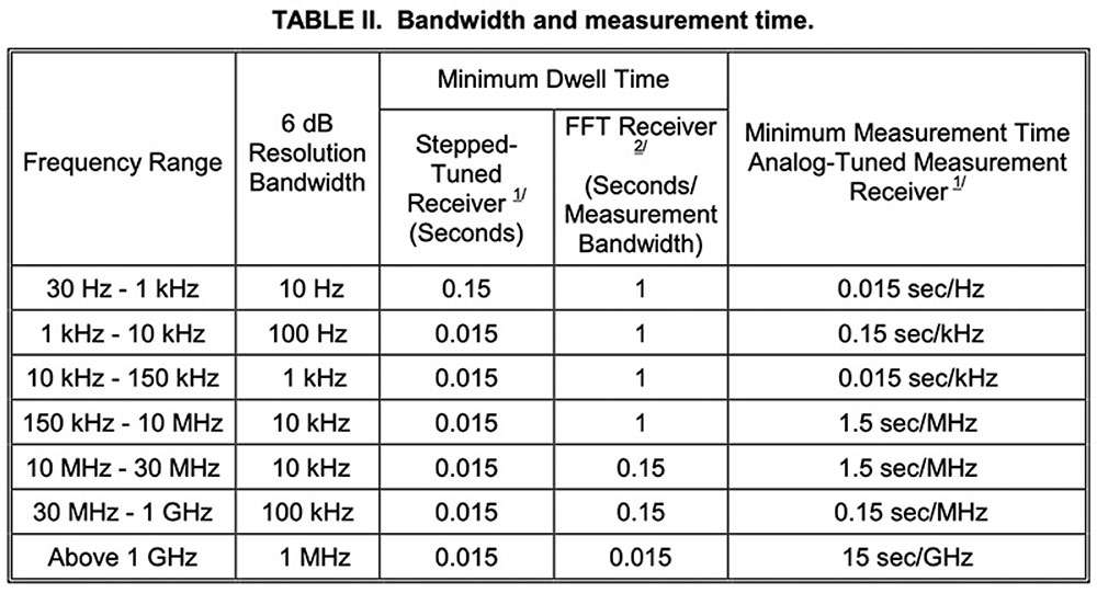
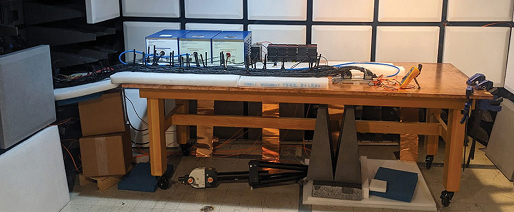
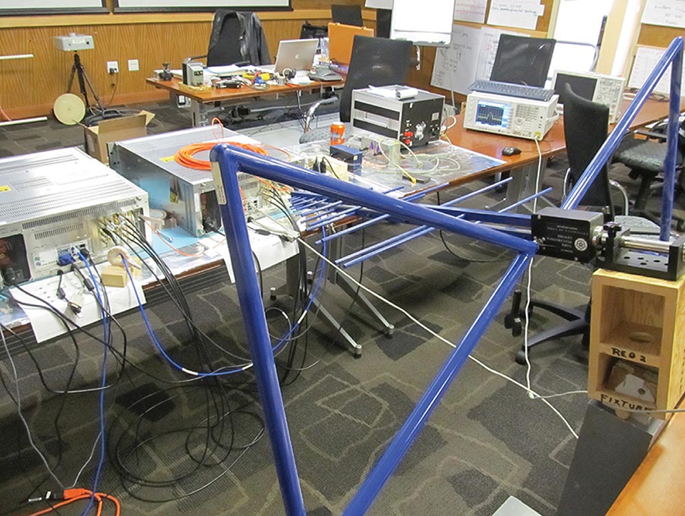
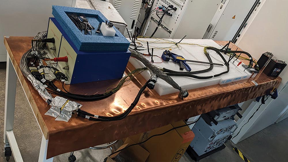
Figure 8 on page 21 shows one of my early MIL-STD-461 test setups for measuring radiated emissions from some aerospace ground equipment. I used heavy-duty aluminum foil taped down to a conference table. Although, I was using a commercial bi-log antenna, the test results still provided me some confidence there were no “red flags” apparent. The product was later tested and passed.
I’ll usually run a baseline plot on the analyzer using “Max Hold” mode for a couple of minutes to build up a composite ambient plot. Then, I’ll activate additional traces for the actual measurements. For example, I often have at least two plots or traces on the screen: the ambient baseline and the actual measurement. It greatly helps to become familiar with your area’s RF spectrum usage.
It’s also a bonus if you already know the top harmonic frequencies because it’s easier to identify product emissions from the ambient noise. I often “zero in” by reducing the frequency span on a high harmonic while performing a measurement.
Fortunately, there are three ways around this:
- In most cases, you’ll observe a range of product emissions in a harmonic relationship. Very often, these harmonics are created from the same source and if one or more are masked by ambient signals, then working on the others that are more visible will generally bring the whole batch down.
- In some cases, there will be a critical harmonic masked by an ambient transmitter. A common example is a 100 MHz harmonic hidden underneath a strong FM broadcast station at the 99.9 MHz channel. In this case, I’ll try reducing the resolution bandwidth from 100 or 120 kHz down to as little as 1 kHz or less. This often “filters out” the modulation from the FM station, allowing you to observe the hidden harmonic. This also presumes the harmonic is an unmodulated continuous wave (CW) signal. Just be sure reducing the RBW doesn’t also reduce the harmonic amplitude. If your harmonic is modulated, this may not work, so you could try selecting a higher related harmonic, as in (1) above.
- Move your testing well away from urban transmitters (easier said than done these days) or test in the early morning hours.
Remember that strong nearby transmitters can affect the amplitude accuracy of the measured signals, as well as create mixing products that appear to be harmonics, but are really combinations of the transmitter frequency and mixer circuit in the analyzer. You may need to use an external bandpass filter at the desired harmonic frequency to reduce the effect of the external transmitter. An example would be an FM broadcast band “stop band” filter.
Making these manual measurements for every dominant harmonic can be tedious at best. In Part 4, I’ll cover some pre-compliance software that will help speed up your test and analysis.
- Wyatt, “EMC Bench Notes: Pre‑Compliance Testing for Radiated Emissions – Part 2: Making the Measurement,” In Compliance website.
- Wyatt, “EMC Bench Notes: Pre‑Compliance Testing for Radiated Emissions – Part 1: Equipment Needs,” In Compliance website.
- Wyatt, EMC Troubleshooting Trilogy, Volume 2.
- Wyatt, “Evaluating Reduced-Size EMI Antennas – Part 1,” EDN.
- Tekbox Roll-Up Ground Plane, Model TGGP.